
Home Sweet Home
A place to feel safe!
Home Sweet Home
A place to feel safe!
(AmsMath Guide in Org – Too late for a headline; just the best I can do for now)
This script is an exercise of amsmath features, and a test for their compatibility with org mode export to html. It mainly reproduces the User Guide 2.1, connected to the latex package amsmath, rev. 2019-10-14. The blog version 2022-08-08 gets sparse beginning with the Section Operator names.
Issues related to the collaboration of org mode, latex, and mathjax are addressed in the text; see the mathjax discussion about ams in the extension list for latex. I'm plan to separate these parts from the mathematical content.
Medium.com and the free version of wordpress don't accept
javascript inclusion, so mathjax is not an
option. For kind of an ugly exception handling I can use the
png export of latex math by setting the option
tex:dvipng. The side effects – and out-ruling arguments – of this
surrogate “depiction” begin to show in the examples of Section
4.6 Equation groups with mutual
alignment:
So, the tex:dvipng solution has to be revisited for being a valuable
solution. Another reason to change the system.
The amsmath package is a latex package that provides miscellaneous enhancements for improving the information structure and printed output of documents that contain mathematical formulas. Readers unfamiliar with latex should consult [1]. If you have an up-to-date version of latex, the amsmath package is normally provided along with it. Upgrading when a newer version of the amsmath package is released can be done via the download link.
This documentation describes the features of the amsmath package and discusses how they are intended to be used. It also covers some ancillary packages, like amsbsy, amsopn, amsxtra, amscd, or amstext.
These all have something to do with the contents of math formulas. For
information on extra math symbols and math fonts, see AMS fonts at
ams.org. For documentation of the amsthm package or
AMS document classes, like amsart or amsbook, see
amsthm or Section AMS Author Handbook in the Author
Resource Center at ams.org.
If you are a long-time latex user and have lots of mathematics in what you write, then you may recognize solutions for some familiar problems in this list of amsmath features:
\sin and \lim, including proper side spacing and automatic
selection of the correct font style and size (even when used in sub-
or superscripts).eqnarray environment to make various
kinds of equation arrangements easier to write.eqnarray).equation environment (unlike eqnarray).The amsmath package is distributed together with some small auxiliary packages:
\text{} command for
typesetting a fragment of text inside a display.\DeclareMathOperator{} for
defining new `operator names' like \sin and \lim.CD environment for simple
commutative diagrams (no support for diagonal arrows).\fracwithdelims{} and
\accentedsymbol{}, for compatibility with documents created using
version 1.1.The amsmath package incorporates amstext, amsopn, and amsbsy. The features of amscd and amsxtra, however, are available only by invoking those packages separately.
The independent mathtools package provides some enhancements to amsmath and loads amsmath automatically. Some mathtools facilities will be noted below as appropriate.
The amsmath package has the following options:
centertags – (default) For an equation containing a split
environment, place equation numbers vertically centered on the total
height of the equation.tbtags – `Top-or-bottom tags': For an equation containing a
split environment, place equation numbers level with the last
(resp. first) line, if numbers are on the right (resp. left).sumlimits – (default) Place the subscripts and superscripts of
summation symbols above and below, in displayed equations. This
option also affects other symbols of the same type — \(\prod\), \(\coprod\),
\(\bigotimes\), \(\bigoplus\), and so forth — but excluding integrals
(see below).nosumlimits – Always place the subscripts and superscripts of
summation-type symbols to the side, even in displayed equations.intlimits – Like sumlimits, but for integral symbols.nointlimits – (default) Opposite of intlimits.namelimits – (default) Like sumlimits, but for certain
`operator names' such as det, inf, lim, max, min, that
traditionally have subscripts
placed underneath when
they occur in a displayed equation.nonamelimits – Opposite of namelimits.alignedleftspaceyes –alignedleftspaceno –alignedleftspaceyesifneg –
To use one of these package options, put the option name in the optional
argument of the \usepackage{} command — e.g.,
For AMS document classes and any other classes that preload
amsmath desired options must be specified with the
\documentclass{}— e.g.,
The amsmath package also recognizes the following options which
are normally selected (implicitly or explicitly) through the \documentclass{}
command, and thus need not be repeated in the option list of the
\usepackage{amsmath} statement.
leqno – Place equation numbers on the left.reqno – Place equation numbers on the right.fleqn – Position equations at a fixed indent from the left
margin rather than centered in the text column.
Three options have been added to control the space to the left of
aligned and gathered environments. Prior to the 2017 release
a thin space was added to the left but not the right of these constructs.
This appears to have been an accidental feature of the implementation and
was typically corrected by prefixing the environments with \!.
The new default behavior is aimed to ensure that the environments do
not have a thin space added in most cases, and that existing documents
using \!\begin{aligned} continue to work as before.
alignedleftspaceyes – Always add \, to the left of aligned and
gathered.alignedleftspaceno – Never add \, to the left of aligned and
gathered.alignedleftspaceyesifneg – Only add \, if the environment is prefixed by
negative space. (New default behavior.)
The amsmath package provides a number of additional displayed
equation structures beyond the ones provided in basic latex. The
augmented set includes align, alignat, equation , flalign, gather,
multline, with asterisk alternative, and split without.
Although the standard eqnarray environment remains
available, it is better to use align or equation & split instead. Within
eqnarray, spacing around signs of relation is not the preferred mathematical
spacing, and is inconsistent with that spacing as it appears in other
environments. Long lines in this environment may result in misplaced or
overprinted equation numbers. This environment also does not support the use of
\qed or \qedhere as provided by theorem packages. |
Except for split, each environment has both starred and unstarred
forms, where the unstarred forms have automatic numbering using
latex's equation counter. You can suppress the number on any
particular line by putting \notag before the end of that line.
\notag should not be used outside a display environment as it will
mess up the numbering.
|
You can also override a number with a tag of your own using \tag{label}, where
label means arbitrary text such as $*$ or ii used to “number” the
equation. A tag can reference a different tagged display by use of
\tag{\ref{label}modifier} where modifier is optional. If you include
hyperref, use \ref*{}; using the starred form of \ref{}
prevents a reference to a modified tag containing a nested link from linking to
the original display.
There is also a \tag*{} command that causes the text you supply to be typeset
literally, without adding parentheses around it. \tag{} and \tag*{} can also
be used within the unnumbered versions of all the amsmath
alignment structures. Some examples of the use of \tag{} may be found in the
sample files 📂 testmath.tex and 📂 subeqn.tex
provided with the amsmath package.
The split environment is a special subordinate form that is used
only inside one of the others. It cannot be used inside
multline, however. split supports only one alignment column, i.e. only one & character; if more are needed, aligned or alignedat should be
used. The width of a split structure is the full line width.
In the structures that do alignment, i.e., split, align, alignat, and
flalign, relation symbols have an & before them but not after — unlike
eqnarray. Putting the & after the relation symbol will interfere with the
normal spacing; it has to go before.
In all multiline environments, lines are divided by \\.
The \\ should not be used to end the last line. Using it
there will result in unwanted extra vertical space following the display.
|
In all math environments, no matter if inline or display, blank lines, or the equivalents to \par, are not permitted, and will result in an error. → See Section 4.9.
|
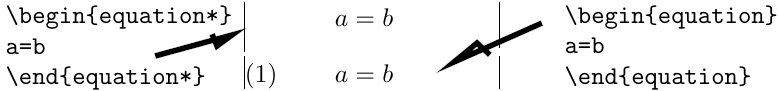
The equation environment is for a single equation with an
automatically generated number. The equation* environment is the
same except for omitting the number.
Basic latex doesn't provide an equation* environment,
but rather a functionally equivalent environment named
displaymath. |
The wrapper \[ ... \] is equivalent to equation*.
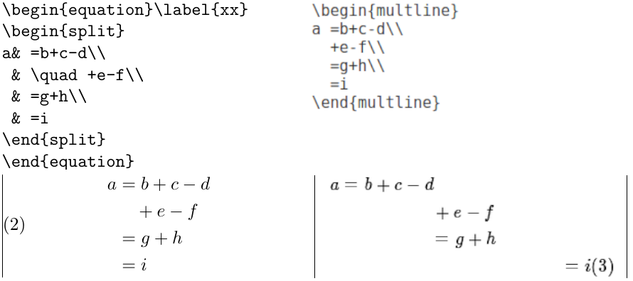
The multline environment is a variation of the equation
environment used for equations that don't fit on a single line. The
first line of a multline will be at the left margin and the last
line at the right margin, except for an indention on both sides in the
amount of \multlinegap{}. Any additional lines in between will be
centered independently within the display width, unless the fleqn
option is in effect.
Like equation, multline has only a single equation number
(thus, none of the individual lines should be marked with \notag).
The equation number is placed on the last line (\opt{reqno} option) or
first line (\opt{leqno} option); vertical centering as for split
is not supported by multline.%
It's possible to force one of the middle lines to the left or right with
commands \shoveleft{}, \shoveright{}. These commands take the entire
line as an argument, up to but not including the final \\; for
example \shoveright{+e-f}\\ would shift the line \(+e-f\) in Figure 2 to the right leaving a virtual gap for the number (3) below.
The value of \multlinegap{} can be changed with the latex
core commands \setlength{}{} or \addtolength{}{}.
Like multline, the split environment is for single equations that are too
long to fit on one line and hence must be split into multiple lines. Unlike
multline, however, the split environment provides for alignment among the
split lines, using & to mark alignment points. Unlike the other
amsmath equation structures, the split environment provides no
numbering, because it is intended to be used only inside some other displayed
equation structure, usually an equation, align, or gather environment,
which provides the numbering. Check the difference in Figure 2.
The split structure should constitute the entire body of the
enclosing structure, apart from commands like \label{} that produce no
visible material.
The gather environment is used for a group of consecutive
equations when there is no alignment desired among them; each one is
centered separately within the text width, see Figure 3.
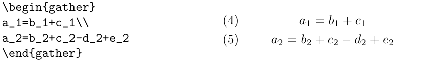
gather amsmath environment
Equations inside gather are separated by a \\ command.
Any equation in a gather may mix with split environments, for example:
\begin{gather} 1st equation \\ 2nd equation \\
\begin{split} 3rd & two \\ & line eqn \end{split} \\
4th equation \\ 5th ... get the picture ... \end{gather}
The align environment is used for two or more equations when
vertical alignment is desired; usually binary relations such as equal
signs are aligned, like in Figure 4.
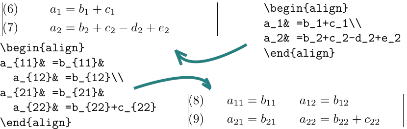
To have several equation columns side-by-side, use extra ampersands to separate the columns:
\begin{align} x&=y & X&=Y & a&=b+c\label{eq:C}\\ x'&=y' & X'&=Y' & a'&=b\label{eq:D}\\ x+x'&=y+y' & X+X'&=Y+Y' & a'b&=c'b \end{align}\begin{align} x&=y & X&=Y & a&=b+c\\ x'&=y' & X'&=Y' & a'&=b\\ x+x'&=y+y' & X+X'&=Y+Y' & a'b&=c'b \end{align}
Line-by-line annotations on an equation can be done by judicious
application of \text{} inside an align environment:
\begin{align}
x& = y_1-y_2+y_3-y_5+\dots && \text{by \eqref{eq:C}}\\
 & = y'\circ y^*           && \text{by \eqref{eq:D}}\\
 & = y(0) y'           && \text {by Axiom 1.}
\end{align}
A variant environment alignat allows the horizontal space between
equations to be explicitly specified. This environment takes one argument,
the number of “equation columns” (the number of pairs of right-left
aligned columns; the argument is the number of pairs): count the maximum
number of ampersands in any row, add 1 and divide by 2.
\begin{alignat}{2}
x& = y_1-y_2+y_3-y_5+\dots &\;& \text{by \eqref{eq:C}}\\
 & = y'\circ y^*             && \text{by \eqref{eq:D}}\\
 & = y(0) y'             && \text {by Axiom 1.}
\end{alignat}
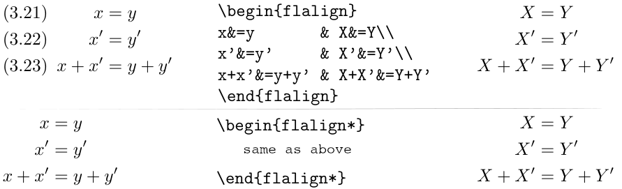
The environment flalign, i.e., full length alignment, stretches the
space between the equation columns to the maximum possible width, leaving
only enough space at the margin for the equation number, if present.
Like equation, the multi-equation environments gather,
align, and alignat are designed to produce a structure
whose width is the full line width. This means, for example, that one
cannot readily add parentheses around the entire structure. But
the variants gathered, aligned, and alignedat are provided whose
total width is the actual width of the contents; thus they can be used
as a component in a containing expression. E.g.,
\begin{equation*}\left.\begin{aligned}
  \frac{\partial B}{\partial t}&=-\nabla\times E,\\
  \frac{\partial E}{\partial t}&=\nabla\times B - 4\pi j,
\end{aligned}\right\}\qquad
\text{Maxwell's equations} \end{equation*}
Like the array environment, these -ed variants also take an optional [t]
top, [b] bottom or the default [c] center option argument to specify
vertical positioning.
| For maximum interoperability, do not insert a space or line break before the option. |
Certain equation environments wrap their contents
in an unbreakable box, with the consequence that neither \displaybreak
nor \allowdisplaybreaks will have any effect on them. These include
split, aligned, gathered, and alignedat.
|
Case constructions like the following are common in mathematics:
\begin{equation} P_{r-j}=\begin{cases} 0& \text{if $r-j$ is odd},\\ r!\,(-1)^{(r-j)/2}& \text{if $r-j$ is even}. \end{cases} \end{equation}
and in the amsmath package there is a cases environment to
make them easy to write:
P_{r-j}=\begin{cases}
    0&  \text{if $r-j$ is odd},\\
    r!\,(-1)^{(r-j)/2}&  \text{if $r-j$ is even}.
  \end{cases}
Notice the use of \text{} – → see Section 6
– and the nested math formulas. The cases environment is set in
\textstyle. If \displaystyle is wanted, it must be requested
explicitly; mathtools provides a dcases environment
for this purpose.
The -ed and cases
environments must appear within an enclosing math environment, which can
be either in text, between $...$, or in any of the display environments.
Placing equation numbers can be a rather complex problem in multiline displays. The environments of the amsmath package try hard to avoid overprinting an equation number on the equation contents, if necessary moving the number down or up to a separate line. Difficulties in accurately calculating the profile of an equation can occasionally result in number movement that doesn't look right.
A \raisetag{} command is provided to adjust the vertical position of the
current equation number, if it has been shifted away from its normal
position. To move a particular number up by six points, write
\raisetag{6pt}.
At the end of a display, the \raisetag{} command also
shifts up the text following the display. |
A \raisetag{} adjustment is fine tuning like line breaks
and page breaks, and should be left undone until your document is nearly
finalized, or you may end up redoing the fine tuning several times to keep up
with changing document contents. |
You can use the \\[dimension] command to get extra vertical space between
lines in all the amsmath displayed equation environments, as is
usual in latex.
Do not type a space between the \\ and the following [;
only for display environments defined by amsmath the space is
interpreted to mean that the bracketed material is part of the document
content. |
When the amsmath package is in use between equation lines are
normally disallowed; the philosophy is that page breaks in such material
should receive individual attention from the author. To get an individual
page break inside a particular displayed equation, a \displaybreak command
is provided. \displaybreak is best placed immediately before the \\ where
it is to take effect. Like latex's \pagebreak,
\displaybreak takes an optional argument between 0 and 4 denoting the
desirability of the pagebreak. \displaybreak[0] means “it is permissible to
break here” without encouraging a break; \displaybreak with no optional
argument is the same as \displaybreak[4] and forces a break.
If you prefer a strategy of letting page breaks fall where they may, even in
the middle of a multiline equation, then you might put
\allowdisplaybreaks[1] in the preamble of your document. An optional
argument 1–4 can be used for finer control: [1] means allow page breaks,
but avoid them as much as possible; values of 2,3,4 mean increasing
permissiveness. When display breaks are enabled with \allowdisplaybreaks,
the \\* command can be used to prohibit a pagebreak after a given line, as
usual.
Certain equation environments wrap their contents in an
unbreakable box, with the consequence that neither \displaybreak nor
\allowdisplaybreaks will have any effect on them. These include split,
aligned, gathered, and alignedat. |
The command \intertext{} is used for a short interjection of one or two
lines of text in the middle of a multiple-line display structure; → see also
Section 6 The text command of the User’s Guide for the amsmath
Package. Its salient feature is preservation of the alignment, which would
not happen if you simply ended the display and then started it up again
afterwards. \intertext{} may only appear right after a \\ or \\*
command. Notice the position of the word “and” in the example depicted in
Figure 6, produced by
\begin{align}
  A_1&=N_0(\lambda;\Omega')-\phi(\lambda;\Omega'),\\
  A_2&=\phi(\lambda;\Omega')-\phi(\lambda;\Omega),\\
\intertext{and}
  A_3&=\mathcal{N}(\lambda;\omega).
\end{align}
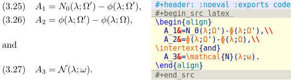
\intertext{} interjection of a text paragraph without breaking the equation alignment. – Right: the org mode source code block for inserting the code of the example.
The mathtools package provides a command
\shortintertext{} that is intended for use when the interjected text is
only a few words; it uses less vertical space than \intertext{}. This is
most effective when equation numbers are on the right. |
In latex if you wanted to have equations numbered within
sections — that is, have equation numbers (1.1), (1.2), …, (2.1),
(2.2), …, in sections 1, 2, and so forth — you could redefine
\theequation{} as suggested in [1]1:
\renewcommand{\theequation}{\thesection.\arabic{equation}}
This works pretty well, except that the equation counter won't be reset to
zero at the beginning of a new section or chapter, unless you do it yourself
using \setcounter{}. To make this a little more convenient, the
amsmath package provides the command \numberwithin{}{}. To
have equation numbering tied to section numbering, with automatic reset of
the equation counter, write
\numberwithin{equation}{section}
As its name implies, the \numberwithin{} command can be applied to any
counter, not just the equation counter. Addition of the blog author:
“… but the results may not be satisfactory in all cases because of potential complications. See the discussion of the
\addtoresetcommand in Subsection A.1.4 Defining and changing counters, Section A.1 Linking markup and formatting of Appendix A LaTeX Overview for Preamble, Package, and Class Writers”
— Subsection 8.2.14 Resetting the equation counter, Section 8.2 Display and alignment structures for equations of [2]'s Chapter 8 Higher Mathematics
To make cross-references to equations easier, an \eqref{} command is
provided. This automatically supplies the parentheses around the equation
number. I.e., if \ref{abc} produces 3.2 then \eqref{abc} produces
(3.2). The parentheses around an \eqref{} equation number will be set in
upright type regardless of type style of the context.
The amsmath package provides also a wrapper environment,
subequations, to make it
easy to number equations in a particular \align{} or similar group with
a subordinate numbering scheme. For example
\begin{subequations}
...
\end{subequations}
causes all numbered equations within that part of the document to be numbered
(4.9a) (4.9b) (4.9c) …, if the preceding numbered equation was (4.8). A
\label{} command immediately after \begin{subequations} will produce a
\ref{} of the parent number 4.9, not 4.9a. The counters used by the
subequations environment are parentequation and equation and
\addtocounter{}, \setcounter{}, \value{}, etc., can be applied as usual
to those counter names. To get anything other than lowercase letters for the
subordinate numbers, use standard latex methods for changing
numbering style; → see, again, Sections 6.3 Numbering, Chapter 6 Designing
It Yourself and Subsection C.8.4 Numbering in Section C.8 Definitions,
Numbering, and Programming, Appendix C Reference Manual of the
latex manual [1]. For example, redefining
\theequation{} as follows will produce roman numerals.
\begin{subequations}
\renewcommand{\theequation}{\theparentequation \roman{equation}}
Note that the \renewcommand has to be placed into the subequations environment, right behind the \begin{} statement. |
The default equation number is set in \normalfont. This means that
in bold section headings, bold is suppressed; a workaround for this is
to use the standard \ref{} with parentheses rather than \eqref{}.
If another font size is specified for a numbered display, the size of the equation number will inherit this size. The default size can be forced throughout a document by applying this patch in the preamble:
\makeatletter
\renewcommand{\maketag@@@}[1]{\hbox{\m@th\normalsize\normalfont#1}}%
\makeatother
This modification may be included in a future version of amsmath.
The amsmath package provides some environments for matrices
beyond the basic array environment of latex. The pmatrix,
bmatrix, Bmatrix, vmatrix and Vmatrix have, respectively, \((\,)\),
\([\,]\), \(\lbrace\,\rbrace\), \(\lvert\,\rvert\), and \(\lVert\,\rVert\)
delimiters built in. For naming consistency there is a matrix environment
sans delimiters. This is not entirely redundant with the array environment;
the matrix environments all use more economical horizontal spacing than the
rather prodigal spacing of the array environment. Also, unlike the array
environment, you don't have to give column specifications for any of the
matrix environments; by default you can have up to 10 centered columns.
The maximum number of columns in a matrix
is determined by the counter MaxMatrixCols, default value .. 10, which you
can change if necessary using latex's \setcounter{}{} or
\addtocounter{}{} commands. |
If you need left or right alignment in a column or other
special formats you may use the array environment, or the
mathtools package which provides starred variants of these
environments with an optional argument to specify left or right
alignment. |
To produce a small matrix suitable for use in text, there is a smallmatrix
environment, e.g., \( \bigl( \begin{smallmatrix} a&b\\ c&d \end{smallmatrix}
\bigr) \), that comes closer to fitting within a single text line than a
normal matrix. Delimiters must be provided. The mathtools
package provides p, b, B, v, and V versions of smallmatrix, as
well as * variants as described above. The above example was produced by
\bigl( \begin{smallmatrix}
  a&b\\ c&d
\end{smallmatrix} \bigr)
\hdotsfor[]{n} produces a row of dots in a matrix spanning the given number
of columns. For example,
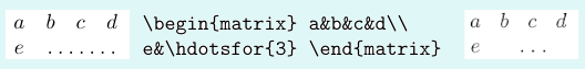
\hdotsfor{n} command at work. With (right) and without (left) colortbl conflicts.
This construct doesn't work with mathjax. Even in
latex there are reported interferences with
colortbl, see stackoverflow entry Interaction between
\hdotsfor and colortbl: Bug or Feature? Results of
this interference are shown in Figure 7, right and
Figure 8, right: the dots just spans a region without the
marginal colums of the specified range. It is described as a conflict
of \fill commands.
If the command works the spacing of the dots can be varied through use of a
square-bracket option, for example, \hdotsfor[1.5]{3}. The number in
square brackets will be used as a multiplier, i.e., the normal value is
1.0. Figure 8, left, shows the effect of spacing two. The matrix
on the right shows the colortbl conflict, and a regular \dots
solution produced by the code
\begin{pmatrix} D_1t&-a_{12}t_2&\dots&-a_{1n}t_n\\
-a_{21}t_1&D_2t&\dots&-a_{2n}t_n\\
\hdotsfor[2]{4}\\ \dots&\dots&\dots&\dots\\
-a_{n1}t_1&-a_{n2}t_2&\dots&D_nt\end{pmatrix}
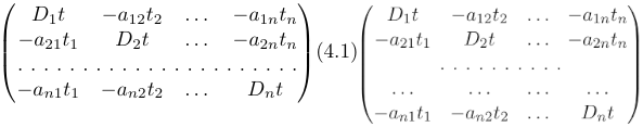
\hdotsfor[2]{4} – Right: colortbl conflict in row three, usage of \dots in every single field of row four.The amsmath package slightly extends the set of math spacing commands, as shown in Table 1. Both the spelled-out and abbreviated forms of these commands are robust, and they can also be used outside of math.
| Macro | Example | Macro | ||
|---|---|---|---|---|
\, |
\thinspace |
\(2\,x\quad 2\!x\) | \negthinspace |
\! |
\: |
\medspace |
\(2\:x\quad 2\negmedspace x\) | \negmedspace |
|
\; |
\thickspace |
\(2\;x\quad 2\negthickspace x\) | \negthickspace |
|
2\quad x |
\(2\quad x\qquad y\) | \qquad y |
||
2\mspace{18mu}x |
\(2\mspace{18mu}x\mspace{-18mu}y\) | \mspace{-18mu}y |
For the greatest possible control over math spacing, use \mspace{}
and math units. One math unit, or mu, is equal to 1/18 em. Thus to
get a negative \quad{} you could write \mspace{-18.0mu}.
For preferred placement of ellipsis dots, raised or on the base line, in various contexts there is no general consensus. It may therefore be considered a matter of taste. By using the semantically oriented commands
\dotsc{} for “dots with commas”\dotsb{} for “dots with binary operators/relations”\dotsm{} for “multiplication dots”\dotsi{} for “dots with integrals”\dotso{} for “other dots” (none of the above)
instead of \ldots and \cdots, you make it possible for your
document to be adapted to different conventions on the fly, in case (for
example) you have to submit it to a publisher who insists on following
house tradition in this respect. The default treatment for the various
kinds follows American Mathematical Society conventions; see the example below, first the code and then its compilation, where the \dot variations are used in the order given by the itemlist above:
Then we have the series \(A_1, A_2, \dotsc\), the regional
sum \(A_1 +A_2 +\dotsb\), the orthogonal product
\(A_1 A_2 \dotsm\), and the infinite integral
\[\int_{A_1}\int_{A_2}\dotsi.\]
Then we have the series \(A_1,A_2,\dotsc\), the regional sum \(A_1+A_2+\dotsb\), the orthogonal product \(A_1A_2\dotsm\), and the infinite integral \[\int_{A_1}\int_{A_2}\dotsi.\]
For most situations, the undifferentiated \dots can be used, and
amsmath will output the most suitable form based on the
immediate context; if an inappropriate form results, it can be corrected
after examining the output.
A command \nobreakdash is provided to suppress the possibility of a line
break after the following hyphen or dash. For example, if you write
“pages 1– 9” as pages 1\nobreakdash--9 then a line break
will never occur between the dash and the 9. You can also use \nobreakdash
to prevent undesirable hyphenations in combinations like $p$-adic. For
frequent use, it's advisable to construct new macros, e.g.,
\newcommand{\p}{$p$\nobreakdash}% for "\p-adic"
\newcommand{\Ndash}{\nobreakdash--}% for "pages 1\Ndash 9"
%    For "\n dimensional" ("n-dimensional"):
\newcommand{\n}[1]{$n$\nobreakdash-\hspace{0pt}}
The last example shows how to prohibit a line break after the hyphen but allow normal hyphenation in the following word. To accomplish this it suffices to add a zero-width space after the hyphen.
In ordinary latex the placement of the second accent in doubled
math accents is often poor. With the amsmath package you will
get improved placement of the second accent, i.e., \hat{\hat{A}} compiles
to \(\hat{\hat{A}}\) and triggers a customization of the line height.
The commands \dddot and \ddddot are available to produce triple and
quadruple dot accents \(\dddot{a}\) and \(\ddddot{a}\) in addition to the
\dot and \ddot accents \(\dot{a}\) and \(\ddot{a}\) already available in
latex.
To get a superscripted hat or tilde character, load the amsxtra
package and use \sphat or \sptilde. Usage is A\sphat. Note the absence
of the superscript operator ^.
To place an arbitrary symbol in math accent position, or to get under accents, see the accents package by Javier Bezos. And make sure to load amsmath before accents.
Sometimes we might not be happy with the default latex placement
of root indices, e.g., \sqrt[\beta]{k} looks like \(\sqrt[\beta]{k}\). In the
amsmath package \leftroot{} and \uproot{} allow you to
adjust the position of the root:
\sqrt[\leftroot{-2}\uproot{2}\beta]{k}
will move the beta up and to the right:
\(\sqrt[\leftroot{-2}\uproot{2}\beta]{k}\). The negative argument used with
\leftroot{-2} moves the \(\beta\) to the right. The units are normalized to a
small amount that is a useful size for such adjustments.
The command \boxed{} puts a box around its
argument, like \fbox{} except that the contents are in math mode, e.g.
is the result of
\begin{equation}
\boxed{\eta \leq C(\delta(\eta) +\Lambda_M(0,\delta))}
\end{equation}
Basic latex provides \overrightarrow{} and \overleftarrow{}
commands. Some additional over and under arrow commands are provided by the
amsmath package to extend to concepts shown in Table
2.
| arrow | over .. text | under .. math |
|---|---|---|
| .. left .. | \(\overleftarrow{\text{wvec}}\) | \(\underleftarrow{wvec}\) |
| .. right .. | \(\overrightarrow{\text{widevector}}\) | \(\underrightarrow{wipeveqtor}\) |
| .. leftright .. | \(\overleftrightarrow{\text{wvec}}\) | \(\underleftrightarrow{wveq}\) |
\xleftarrow{} and \xrightarrow{} produce
arrows that extend automatically to accommodate
unusually wide subscripts or superscripts. These commands take one
optional subscript argument and one superscript argument:
A\xleftarrow{\overrightarrow{n+\mu-1}}%
B\xrightarrow[T]{n\pm i-1}%
C\xrightarrow[?]{\overleftarrow{\mspace{36mu}}}%
D\xrightarrow[\text{sunrise}]{}E
Here mathjax provides only some idea of the concept, while the latex compilation seems to include more layout considerations.
latex provides \stackrel{} for placing a superscript above a
binary relation. In the amsmath package there are somewhat
more general commands, \overset{} and \underset{}, that can be used to
place one symbol above or below another symbol, whether it's a relation or
something else. The input \underset{*}{X} is compiled to
\(\underset{*}{X}\) while \overset{} is the analog for adding a symbol
above like \(\overset{*}{X}\). The command \overunderset{o}{u} is a
combination of these, taking three arguments to place superscript sized
expressions above and below the same base.
In the paragraph above we can see that these under- and overscripts both add some line height. So it's probably not a good idea to use these commands inline.
The main use of the command \text{} is for words or phrases in a
display. It is very similar to the latex command
\mbox{} in its effects, but has a couple of advantages. If you want
a word or phrase of text in a subscript, you can type |…\textrm{word
or phrase}|, which is slightly easier than the \mbox{} equivalent:
..._{\mbox{\rmfamily\scriptsize word or phrase}}. Note that the
standard \textrm{} command will use the amsmath
\text{} definition, but ensure the \verb+\rmfamily+ font is used.
Supplements of this posting: I provide the pdf here at pjs.netlify.app and a reduced version of the org source at bitbucket.org.
| [1] | Leslie Lamport. LaTeX. Addison-Wesley, 2nd edition, 1994. [ bib ] |
| [2] | Frank Mittelbach, Michel Goossens, Johannes L. Braams, David P. Carlisle, and Chris A. Rowley. The LaTeX Companion 2. Tools and Techniques for Computer Typesetting. Addison-Wesley Professional, Reading, Massachusetts, second edition, April 2004. [ bib ] |