
Home Sweet Home
A place to feel safe!
Home Sweet Home
A place to feel safe!
(Twinkle ChucK – Too late for a headline; just the best I can do for now). Finished 2023-02-07, published 2023-09-26.
The babel section of org mode delivers all means to act as the control center for composing just anything: slide show, presentation, song, movie, 3D printing; any kind of process control. Here's the part about music with the main focus of translating a basic chuck composition to a musical score in lilypond with R analysis tools in a gnu linux environment. The appendices expand on chuck matters. Is this a way to Memphis?
The concepts of [6]'s first Chapter Basics: Sound,
Waves, and ChucK Programming are condensed in
📂 Listing1.20.ck available at github. It
defines two patches, i.e. sound signal chains, two float, and one
dur variable.
// Twinkle, with two oscillators!
SinOsc s => dac;             // (1) Sine wave oscillator.
TriOsc t => dac;             // (2) Another oscillator (triangle wave).

// our main pitch variable
110.0 => float melody;       // (3) Sets initial pitch.

// gain control for our triangle wave melody
0.3 => float onGain;         // (4) Gains for note on.

// we'll use this for our on and off times
0.3 :: second => dur myDur;  // (5) Notes duration.
Then it initializes both voices – the melody with a gain of onGain,
the bass with 0 – and increases the frequency of the melody, i.e., the
TriOsc instance t, from 110 to \(220\,\text{Hz}\) in
\(1\,\text{Hz}\) steps of \(10\,\text{ms}\) resulting in a duration of
onGain => t.gain;            // (6) Turns on triangle oscillator.
0 => s.gain;                 // (7) Turns off sine osc.

while (melody < 220.0) {     // (8) Loops until pitch reaches 220.
    melody => t.freq;
    1.0 +=> melody;          // (9) Steps up pitch by 1 Hz.
    0.01 :: second => now;   // (10) Every 1/100 of a second.
}
In the context of the book's chapter the technical advancement of this
code snippet is the realization of a “sweeping pitch upward” by using
a while loop.
The next loop is a for loop and advances the time 0.6 seconds twice for both voices and switches the melody note on and off.
// turn both on, set up the pitches
0.7 => s.gain;               // (11) Now turn on sin osc too.
110 => s.freq;               // (12) ...and initialize its pitch.

// play two notes, 1st "Twinkle"
for (0 => int i; i < 2; i++) { // (13) Use a for loop to play two notes.
    onGain => t.gain;        // (14) Turn on triangle.
    myDur => now;            // (15) Let note play.
    0 => t.gain;             // (16) Turn off triangle.
    myDur => now;            // (17) Silence to separate notes.
}
This loop is repeated three times. The result of the first for loop:
the bass plays a \(110\,\text{Hz}\) sine wave with a volume od 0.7
while the triangle wave puts two 0.3-gain melody stacatto quarters of
\(220\,\text{Hz}\) above it. The second for loop is prepared by
another set of frequencies for melody and bass
138.6 => s.freq;            // (19) Sets up next "twinkle" frequency.
1.5*melody => t.freq;
| From these sets of frequencies I can't guess the note names. I could look them up in tables. chuck offers frequency to midi conversion. To get the pitch from a frequency I'll introduce the R packages seewave, soundgen, tabr, and tuneR in Section 3. In the current section I just finish collecting all frequencies and durations used in the sequence. |
The frequencies of the bass line and the next two quarters for the word “little” are set by
146.8 => s.freq;            // (20) Sets up next frequency for "little".
1.6837 * melody => t.freq;
They are again played with the same for loop. Bass and melody for the word “star” is set and played by
138.6 => s.freq;            // (22) Sets up next frequency for "star".
1.5*melody => t.freq;
onGain => t.gain;           // (23) Plays that note...
second => now;              // (24) ...for a second.
The sequence is terminated by decreasing the frequency of the TriOsc
instance t from 330 to \(0\,\text{Hz}\) in \(1\,\text{Hz}\) and in
parallel the SinOsc instance s from 440 to \(0\,\text{Hz}\) in
\(1.333\,\text{Hz}\) steps per \(10\,\text{ms}\), i.e. a duration of
for (330 => int i; i > 0; i--) {  // (25) Uses a for loop to sweep down from 330 Hz.
    i => t.freq;
    i*1.333 => s.freq;
    0.01 :: second => now;  // (25) Uses a for loop to sweep down from 330 Hz.
}
Table 1 shows the single steps. I tried to design it to illustrate some kind of symmetry. The playing time adds up to a total of exactly 9.0 seconds.
| t | 0 | 0 | 1.1 | 1.4 | 1.7 | 2 | 2.3 | 2.6 | |
|---|---|---|---|---|---|---|---|---|---|
| \(\Delta{}t\) | → | 1.1 | 0.3 | 0.3 | 0.3 | 0.3 | 0.3 | 0.3 | |
| mel | – | 110\(\nearrow\)220 | 220 | – | 220 | – | 330 | – | |
| bas | – | – | 110 | % | % | % | 138.6 | % | |
| ↓ | |||||||||
| t | 9.0 | 5.7 | 4.7 | 4.4 | 4.1 | 3.8 | 3.5 | 3.2 | 2.9 |
| \(\Delta{}t\) | ← | 3.3 | 1 | 0.3 | 0.3 | 0.3 | 0.3 | 0.3 | 0.3 |
| mel | 0 | 0\(\swarrow\)330 | 330 | – | 370.41 | – | 370.41 | – | 330 |
| bas | 0 | 0\(\swarrow\) 440 | 138.6 | % | % | % | 146.8 | % | % |
The R packages I mentioned above offer tools related to sound. I've collected a few items about these packages with a focus on frequency-to-notename conversion. As the first entry I also mention an emacs solution. The first seewave list item presents the Math for equal temperament. For me the last, not least at all, entry tabr is a very recent discovery.
calc mode2 of
the emacs calculator is switched on and off by
C-x * c. In this mode the user can
enter a frequency value with a unit introduced by the algebraic-mode
apostrophe selector as ' 440 Hz [RET], then hit l
s (ell .. ess) to get A_4 representing the scientific
pitch notation. The usage of the emacs calculator for
the frequency estimation is demonstrated in the next list item about
seewave in Table 2.
The R package seewave doesn't provide
frequency-to-notename conversion, but the seewave
author's book [14] discusses some
alternatives3 and the documentation of notefreq() shows
the equation for equal temperament, which could be solved for n
to get something like a freqnote() function.
The function notefreq() accepts (1) a note n
entered as a number or as a string like Ab, B, or C#, (2) an
octave index i, and (3) a ref frequency r. The resulting
frequency f is
Approximated with an accuracy of six significant numbers. Table 2 shows the emacs calculator keystrokes for \(1/(2^{3}\sqrt[12]{2^{10}})\) in the frequency estimation.
| keystrokes | result |
|---|---|
1[RET]12[RET]/ |
→ 0.0833333333333 |
2[RET]10[RET]^ |
→ 1024 |
[TAB]^ |
→ 1.78179743628 |
8[RET]* |
→ 14.2543794902 |
1[RET][TAB]/ |
→ 0.0701538780196 |
For the default i=3 the function can be reduced to
For C3 with \(n=1\) that's 261.626 or the F♯3 from Table 3 the \(n=7\) delivers 369.994. According to the corresponding code the chuck'ers offer 370.414. Cool, I've gathered enough knowledge to enter the nitpicking stage.
For the note A3 which has a rank of \(n=10\) I can reduce the first term's \(n-10\) to 0 and with \(a^{0}=1\) this reduction is further simplified to \(f=r\), with an r default of 440.
With the help of these elaborations the dear reader might figure out any frequency with a handheld calculator. Note that the rank number n is neither confined to the range \([1..12]\) nor to integers.4 So, for example, it can map to any of the semitone functions below. Potential decimal parts are representing the musical cent unit which is supposed to change the logarithmic distance of two consecutive notes into a hundred equidistant pieces.
octaves(f,b,a) and returns the
frequency values of b octaves below and a octaves above a
specific frequency f; octaves(220, b=1,a=2) gives the numeric
vector 110 220 440 880 – bold emphasis added.notesDict the user can turn a
soundgen semitone into a pitch.
tuneR .. noteFromFF() returns an integer
valued semitone difference to A3.5 The function noteFromFF()
transforms the frequency value x to the integer valued 12th root
of a frequency-to-diapason relation including a logarithmic tweaking
variable roundshift.
notesFromFF <- round(12 * log(x / diapason, 2) + roundshift)
For example, the frequency \(493\,\text{Hz}\)
yields 2, the B note of the third octave or b'.
The notenames() function translates this numeric
difference to a note name's string like c'. Moreover the function
lilyinput() – and a data-preprocessing function
quantMerge() – can prepare a data frame to be presented as
sheet music by postprocessing with the lilypond. The
lilyinput() help includes a maturity caveat. For
this purpose the features of tabr seem much more
advanced.
tabr .. freq_pitch() turns a frequency
into a pitch. With the parameter octaves the user can choose
tick or integer output, the accidentals can be set to flat
or sharp, and a4 is offered to be set to something different
from the default of 440. A vector input can be collapse'd.
tabr defines its semitones along the midi
numbers. The corresponding freq_semitones() function
delivers numbers with expanded range above 127 and below 0.
Table 3 shows a selection of the R functions. The
corresponding R code starts from the values in the chuck
script 📂 Listing1.20.ck. The rows of Table 3
are
freq_pitch()'es, which match the
lilypond representationfreq_pitch()freq_semitones() that represent the
midi valuesnotesDictf <- c(110,138.6,146.8,220,1.5*220,1.6837*220,440); n <- tuneR::noteFromFF(f); p <- tuneR::notenames(n); t <- tabr::freq_pitch(f,ac="sharp"); i <- tabr::freq_pitch(f,ac="sharp",o="integer"); s <- round(tabr::freq_semitones(f)); g <- round(soundgen::HzToSemitones(f)); d <- soundgen::notesDict[1+g,1]; rbind(Hz=round(f,1),tuneR=p, tfpt=t, tfpi=i, midi=s, sghs=g, sndp=d)
| Hz | 110 | 138.6 | 146.8 | 220 | 330 | 370.4 | 440 |
|---|---|---|---|---|---|---|---|
| tuneR | A | c# | d | a | e' | f#' | a' |
| tfpt | a, | c# | d | a | e' | f#' | a' |
| tfpi | a2 | c# | d | a | e4 | f#4 | a4 |
| midi | 45 | 49 | 50 | 57 | 64 | 66 | 69 |
| sghs | 93 | 97 | 98 | 105 | 112 | 114 | 117 |
| sndp | A2 | C#3 | D3 | A3 | E4 | F#4 | A4 |
In formal music the first event of the Twinkle impro, the upward pitch, already leads into trouble. It has to be related to the song it is part of. How long is it compared to a quarter note of the song's rhythm? How do I translate the subsequent sound constructions of the chuck script to beats and bars?
To get a clue I first go to the score of the Twinkle song at
musescore.com or musicsheets.org. These pages trigger some other
thoughts about the piece of music and the composer's
intentions. musicsheets.org identifies the two names W.A. Mozart and
C.E. Holmes, an Andante tempo of 100 quarters per minute, and a B♭
major key for 14 instruments extended by some snare-basedrum
percussions. While the musescore.com example is an “easy” version in
C major with two voices. The wikipedia
entry for Twinkle confirms the C major key.
Usually the key of a song can be derived from the pitch of the last
melody note. In the case of Twinkle the melody also begins with this
root note. The chuck composers choose the frequency
\(220\,\text{Hz}\), i.e., an A_3 in scientific pitch notation. They,
however, introduce a “main pitch variable” as melody and assign a
value of \(110\,\text{Hz}\) to it. This melody frequency doesn't
show up in the melody, only in the decorations of the snippet and in
the bass line.
Comparing the chuck sequence illustrated by Table
1 to both scores at musescore.com and musicsheets.org a
quarter note is 0.6 seconds and the quarter notes of the melody are
played staccato.6 For the tempo
information near the clef I choose quarters per minute; see
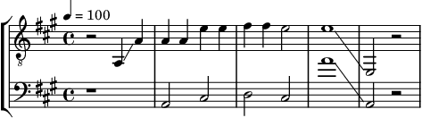
Figure 1. If one quarter takes 0.6 seconds one minute
contains …
For the melody I use a treble or G clef transposed one octave down, the bass line is fine with a bass clef. The glissandi need some more effort. And the duration of the last Twinkle melody note has to be fit in somehow. In the order of appearance I discuss three topics.
The decreasing unit after the short last note raised the question if I should construct the glissandi to be parallel or should I exactly reproduce the downward pitches no matter of their musical context? What about the fact that the upper decrease is played with the bass wave, and the lower one with the melody wave?
The end sequence with two \(3.3\,\text{s}\) downward glissandi can be matched to five quarters plus one quaver. I expand this duration to one and a half note, so the relation from up to downward pitch is maintained. The whole sequence then takes exactly four bars.
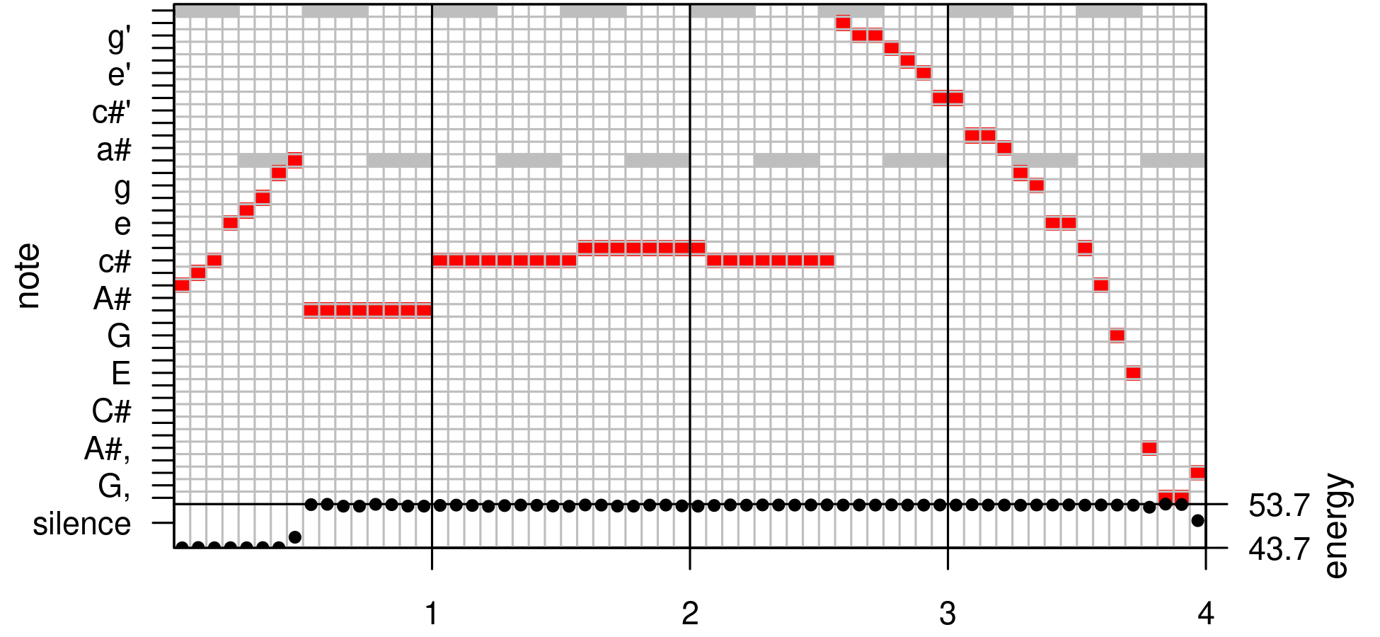
The downward pitches ar much harder to translate. Each of the final glissandi ends with \(0\,\text{Hz}\); nobody can hear or play that. For an exact replication of both glissandi I'd have to calculate the time when the glissando which controls the loop from \(330\,\text{Hz}\) to \(0\,\text{Hz}\) arrives at, say, C0, i.e., \(\approx16.35\,\text{Hz}\). And transfer this result to the glissando from \(440\,\text{Hz}\) to \(0\,\text{Hz}\) which probably leads to a slightly later moment, I guess. The time series illustration in Figure 2 only shows the moment for the fundamental frequency of the whole sound, i.e. the louder bass line.
I decide to call the situation indeterminable and interpret the glitches as glissandi beginning at \(330\,\text{Hz}\) E4 and \(440\,\text{Hz}\), A4. I construct them to be parallel and to consume a range of two octaves, which end at E2 or A2, respectively. The bass-above-melody issue stays untouched.
The lilypond code below generates the sequence shown in
Figure 1. From C3 upwards the lilypond
note names match the tuneR output of
notenames(), while the lilypond
declarations a,|a,,|a,,,|a,,,, translate to A|A,|A,,|A,,, in
tuneR. The lilypond script below should be
reproducible after studying the sources in the Learning7 and the Notation Manual.8'9'10'11'12 Then – after
installing lilypond, including it as babel source code
language in the 📂 .emacs file,13 and getting the
lilypond helpers for emacs14 – with the listing named #+Name: lst1-20muProScore in the
org source, available at bitbucket, the interested reader
can get an impression of lilypond at work in an
org mode source block with the :noweb feature applied.
\parallelMusic melody,base
    { \tempo 4 = 100
    % bar 1                   % bar 2
    r2  a,4\glissando a       a4     a      e'  e' |
    r1                        a,2           cis    |
    % bar 3                   % bar 4
    fis'4  fis'   e'2         e'1\glissando e,2 r2 |
    d             cis         a'1\glissando a,2 r2 |
  }
    \new StaffGroup <<
      \new Staff { \clef "treble_8" \key a \major \melody }
      \new Staff { \clef bass       \key a \major \base }
    >>
To configure a short score snippet without the lilypond
default of a surrounding page like shown in Figure 1 I
included a preamble with the :noweb switch. The Notations Manual's
Spacing Issues Chapter15 deals with the value of its page-breaking
attribute. While the markup settings are part of the Chapter General
Input and Output.16
\version "2.20.0"
\paper{page-breaking = #ly:one-line-breaking
  indent=0\mm        %  line-width=170\mm
  oddFooterMarkup=##f   oddHeaderMarkup=##f
  bookTitleMarkup=##f   scoreTitleMarkup=##f }
Developing the skills for managing lilypond in emacs may take years but I think I named all the essential parts for this special purpose.
For the graph in this section I use results from Section 7 which analyzes the wav file produced in the
next section. Note that this section, Frequency-versus-Time Graph,
doesn't reproduce the fine-tuned musical score from the previous
section. Instead it gets frequency and time information from the
recorded output of the original 📂 Listing1.20.ck
employing the tuneR function FF() without
further explanation. Section 7 then delivers more
insight but still doesn't touch much of the theoretical basics.
The inspiration for this section is to find a programmatic counterpart
of ableton's warping feature or its
audio-to-midi converter. audacity offers
similar ideas in its beat finder, regular interval labels, and label
track at manual.audacityteam.org. And methods outlined by Advances
in Musical Information Retrieval [10] deliver much more
inspiration.
The attribute “frequency versus time” should lead to the undecorated appearance of a piano roll, of illustrating a song like a Gantt Diagram. The common nominator for the illustration of timely events like music is something in the realm of time series. Time series usually concentrate on continuous signals with high data or sampling rates resulting in immense data traffic. Reducing this sea of data to events made the atari notator the tool for the digital evolution of musical ambitions.
| In contrast, expanding the realm of digital
workstations to real time sound design makes the current software
constructions eating up every bit of memory they manage to
grab. Freezing the results of this additional work has become a main
feature of the software. With this procedures the software could be
scaled back to on and off events with dynamic settings and probably
run easily on a 8086 processor or an arduino. For chuck
the users can compare their expectations of the software in the
virtual machine processes, discussed in 3.5 Properties of
[15]'s ChucK Chapter and introduced by Section 3.4
System Design and Implementation.
I consider wavetable synthesis as a link between freezing and in-situ processing. Its purpose is introduced in Section 2 The Evolution of Sound Synthesis of Peter Manning's contribution [8] to Dean's Oxford Handbook of Computer Music: “The processing overheads involved in repeatedly calculating each waveform sample from first principles are significant, and it occurred to Mathews that significant savings could be produced in this regard by calculating the required waveform only once and then using a suitable table lookup procedure to extract this information as the required frequency.” Manning is referring to Mathew's Technology of Computer Music [9]; no specific passage. |
For a start I'll enjoy the graph and discover the data for note-on and note-off events. On the way I hope to get some hints for control parameters in sound design or for note decorations. The graphs melodyplot(), quantplot() and their data are the targets of the event task. The process should motivate digging deeper into Fourier and spectral analysis.
The frequency versus time plot in Figure 2 is made with the help of periodogram() and FF(). With an anticipation of Section 7 about the main tuneR example it delivers 774 frequency values for my wav file. I don't ask why.
All I need the 774 parts for is to construct a proper time series. The
plot() function recognizes the time series and
connects to plot.ts(). The experienced
org mode babbler knows how to transform these lines into
a png plot and include it in this document; see the
org source of this blog entry at bitbucket.
oldPar <- par(mar=c(2,2,0,0)+0.1);
plot(ts1.20,type="h",col="grey85");
abline(h=c(110,220,440),col="grey50",lty="dashed");
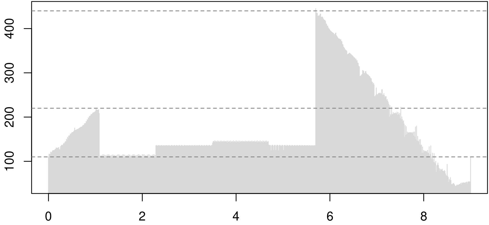
Listing1.20.ck with a series of tuneR functions. They detect the louder bass line and the upward glissando at the start.While the time series class delivers an appropriate plot, the usual time series functions seem unappropriate for making an event list, but I'm not an experinced time series analyst. I'll go with exploratory data analysis. Provided with the graphical feedback I can read 6 ranges into the raw data. The limit indices of the ranges indicate time data; each second contains \(774/9=86\) values, that's about \(11.6\,\text{ms}\) per value. The first and the last range can be least square fit to linear slopes, the other four ranges can be feed into boxplots. Then I can change the parameters of periodogram() or FF() systematically to see the effects.
The code below shows the patch line definitions from the
chuck script 📂 lst1-20rec.ck which records
to 📂 lst1-20rec.wav. It produces a mono track at the
left channel.
| The analysis below in Section 7 prefers to recognize the bass line. For now there are enough procedures to discover, so I don't offer the procedures to split the melody and the bass line to different channels. It's more interesting to discover the functions' preference for the bass line. Stereo sound is one topic of [6]'s second chapter. |
First I have to change the patch lines. The original file
📂 Listing1.20.ck begins with
SinOsc s => dac;             // (1) Sine wave oscillator.
TriOsc t => dac;             // (2) Another oscillator (triangle wave).
For recording I put the SinOsc instance s through the Gain
instance named master into the WvOut sound buffer instance named
w which then disappears in the blackhole nirwana. Then I can
connect the melody line to the master track.
SinOsc s => Gain master => WvOut w => blackhole; // (1) melody chain
TriOsc t => master;                              // (2) bass chain
After that I copy the definitions of the variables melody, onGain,
and myDur and the settings of the .gain attributes for melody and
bass lines. This is exactly like in 📂 Listing1.20.ck,
line 7-21, so I can insert these lines without comments and don't show
them here.
The next part prepares for recording. It reads the current path of the
record script, names the output file, connects path and file name,
assigns the result to the .wavFilename attribute of the WvOut
instance w, and finally turns on the .record feature of w.
me.dir() => string path;             // (3) get file path
"/lst1-20rec.wav" => string fileRec; // (4) target file
path+fileRec => fileRec;             // (5) add the path
fileRec => w.wavFilename;  // (6) choose the record file
w.record(1);               // (7) press the record button
After inserting the rest of 📂 Listing1.20.ck, line
22-end, the recording has to be finished and the file to be closed.
w.record(0);   // (8) press the stop button
w.closeFile;   // (9) close the record file
For invoking chuck in linux it's important to set the sampling rate to \(44100\,\text{Hz}\); on linux the default is \(48\,\text{kHz}\).
cd musRoot/chuck
chuck --srate44100 lst1-20rec.ck
The patch ending in the blackhole still takes as long as the regular
output to dac. But there's a tremendous time warp for using the
--silent option.
cd iMuMy/Chuck
chuck --srate44100 --silent lst1-20rec.ck
Both execute the task properly but terminate with a warning. I think I
recognized this warning generally in the context of using WvOut, but
it also maybe with LiSa or generally with sound buffers.
terminate called without an active exception
Aborted (core dumped)
Timing the commands confirms my manual measurement of 11 seconds. And it shows \(0.4\,\text{s}\) for the silent version.
| time | blackhole | +silent |
|---|---|---|
| real | 0m10,873s | 0m0,408s |
| user | 0m0,573s | 0m0,124s |
| sys | 0m0,351s | 0m0,005s |
For filing I compress the resulting wave file to flac. After taping I've got three new files to work with. A 3k chuck script, a 794k wav, and a 246k flac file. And I'm all set for the …
I refrained from calling this section “sound analysis” because it just
provides a coarse introduction to collected tools without scientific
distraction. The collection is a set of functions picked from the main
example for tuneR.17
I've chosen tuneR instead of seewave, because
tuneR seems closer to the programmatic background. While
seewave offers plenty of parameters to avoid the ...
channel to the underlying functions and includes switches for optional
plots it also makes it hard to customize very basic settings, because
it hides the structure. Meaning that – for the matter of skill
building – I prefer tuneR's unix like aproach
of many small programs to the highly integrated seewave
solutions. After this learning phase I will probably acccept
seewave's help. I don't asssume this as a better way,
it's just my way; greetings from Frank Sinatra.
On my way to a notation compatible with lilypond I skip some distractions from the tuneR example. I don't
In the subsections I look at tuneR plots and I offer some
bridges which are about to help me arriving at sound design. The code
below delivers the data for the rest of the main tuneR
example, employing the functions readWave(),
normalize(), mono(), periodogram(),
FF(), noteFromFF().
tmpfile <- "./iMuMy/Chuck/lst1-20rec.wav";
wn1.20 <- tuneR::normalize(tuneR::readWave(tmpfile));
wnm1.20 <- tuneR::mono(wn1.20, "left"); # str(wSpec);
wSpec <- tuneR::periodogram(wnm1.20, normalize=TRUE,
                            width=1024, overlap=512);
ff <- tuneR::FF(wSpec); # print(ff); str(ff)
notes <- tuneR::noteFromFF(ff, 440);
| Unfortunately the main example for tuneR
is unsufficiently commented. Comments usually come as a tautology like
“the function periodogram() produces a periodogram.”
Fortunately the author of [14] seems to follow
the same track18 without explicitly referencing the main
tuneR example but with more detailed explanations. At
least he follows the line of applying periodogram(),
FF(),19]
noteFromFF(), notenames(),
melodyplot(), quantize(), and
quantplot(). He puts these tuneR functions
into a dominant and fundamental frequency context's comparison of
|
In the main tuneR example normalize() and
mono() prepare the data for
periodogram(). What are these functions doing and to
what degree are they essential for the process?
normalize() turns the \(16\,\text{bit}\) integer values of the amplitude from a range of \(\pm32767\) or \(\pm(2^{16}-1)\), into a real-valued range of \([-1,+1]\). And it centers the values which has the effect that the mean of all values is leveled to zero. To make it comparable to the original wave I multiply the result with 32760, the maximum value of input wave; see Table 4. Is it needed to deliver a real-valued range for the subsequent functions? For the \([-1,+1]\) range? For amplification? Got a distant feeling that it might be helpful for the amplitude envelope discussed in Section 7.5. Just listillo guesses.
tmpfile <- "./iMuMy/Chuck/lst1-20rec.wav";
wv <- tuneR::readWave(tmpfile); # str(wv)
wn <- tuneR::normalize(wv);
rbind(wav=summary(wv@left),norm=round(32760*summary(wn@left)));
| Min. | 1st Qu. | Median | Mean | 3rd Qu. | Max. | |
|---|---|---|---|---|---|---|
| wav | -32751 | -13625 | 113 | 16.62 | 13426 | 32760 |
| norm | -32760 | -13638 | 96 | 0 | 13406 | 32736 |
The mono() function selects a specific channel. It will be more
useful after I put the bass line into a different channel than the
melody, which might deliver some ideas about a “master file”,
equivalent to a master tape. tuneR's multi channel wave
class WaveMC supports more than two
channels. MCnames() defines labels and names for 18
channels derived from an unresolvable link to microsoft's
wav format in the help file.21
The attributes of periodogram() are impressive but I
don't really know how to use them. The help page uses spectral
density as a synonym; doesn't ring a bell either. For now I just see
that periodogram() produces a Wspec class which is
required to feed into the next function FF() to
produce a series of fundamental frequencies. Without deep knowledge
I just have a look at the structure of my recording's Wspec
instance which I ingeniously call wSpec:
Formal class 'Wspec' [package "tuneR"] with 13 slots
  ..@ freq     : num [1:512] 43.1 86.1 129.2 172.3 215.3 ...
  ..@ spec     :List of 774
  .. ..$ : num [1:512] 0.0783 0.3776 0.4763 0.0349 0.0111 ...
  .. 773 similar lines ................
  ..@ kernel   : NULL             ..@ df       : num 2
  ..@ taper    : num 0            ..@ width    : num 1024
  ..@ overlap  : num 512          ..@ normalize: logi TRUE
  ..@ starts   : num [1:774] 1 513 1025 1537 2049 ...
  ..@ stereo   : logi FALSE       ..@ samp.rate: int 44100
  ..@ variance : num [1:774] 0.0285 0.0304 0.0295 0.0281 ...
  ..@ energy   : num [1:774] 43.5 43.9 43.8 43.4 44.1 ...
Shortly after producing this Wspec class tuneR's main
example mentions two graphical illustrations of it:
tuneR::image() a version of the graphics function
image(). It looks distantly related to a
Gantt diagram; the help page calls it spectrogram. According to
the source file it uses wSpec@starts for the x axis,
wSpec@frequ for y, and wSpec@spec for the color.tuneR::plot() a version of the base function
plot(). It produces something like a frequency
spectrum by addressing one of 774 bins by a which
parameter. According to the source file it uses wSpec@freq for the
x axis and wSpec@spec[[which]] for y.
The description at the corresponding plot-WspecMat help says “plotting
a spectrogram (image) of an object of class Wspec or WspecMat. The
usage, too. The tuneR related plot() is an S4 method
for signature WspecMat,missing and image() is for Wspec.” while
the details tell the user that “calling image() on a Wspec object
converts it to class WspecMat and calls the corresponding plot()
function. Calling plot() on a WspecMat object generates an
image() with correct annotated axes.” I find that
confusing. Nevertheless I can apply the illustrations to my Wspec
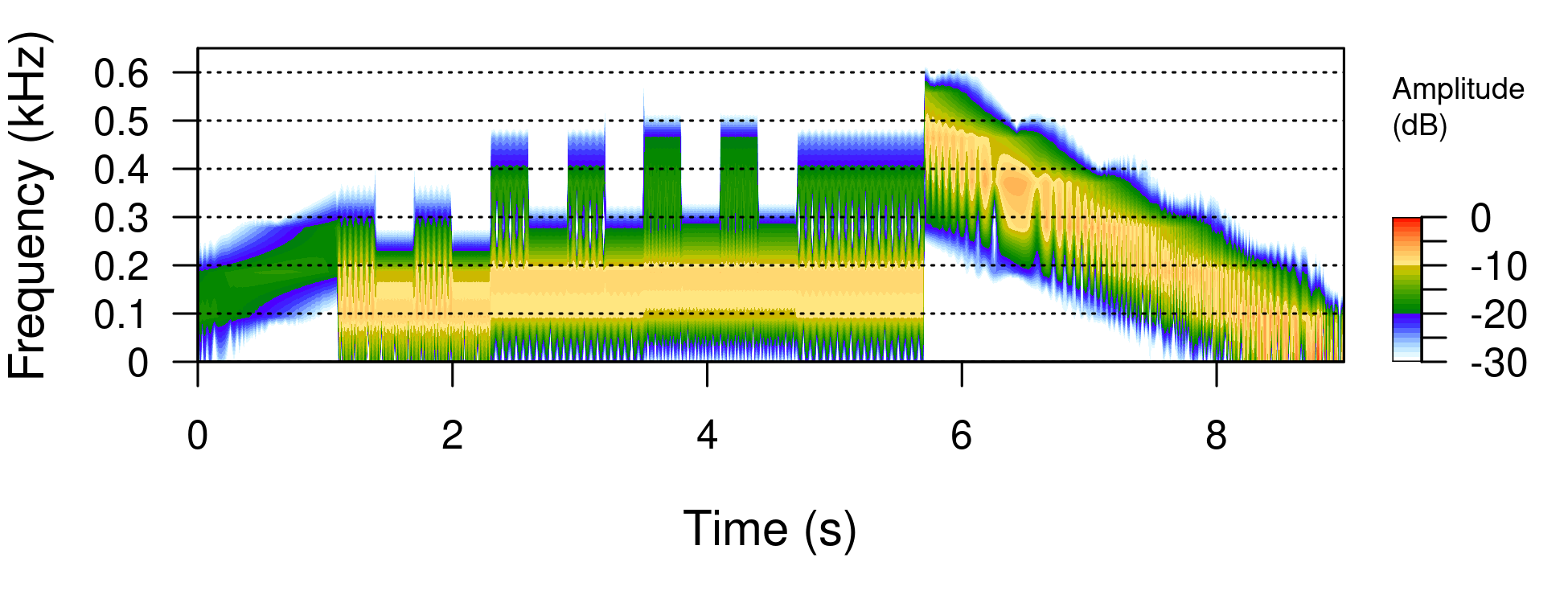
instance wSpec. The code below turns wSpec into Figure
3. Obviously it uses image().
par(mar=c(2,4,0.6,0)+0.1);
tuneR::image(wSpec, ylim=c(0, 500), xunit="time",
             col=c(rep("#FFFFFF",10),rainbow(200)[0:134]));
#            col=seewave::spectro.colors(20));
s <- c(108,133,158,184); t <- s*9/774;
abline(v=t,lwd=0.4,lty="dashed");
text(t,355,paste0("wSpc(",s,") at ", round(t,2), "s"),
     a=c(0.4,-0.45),cex=0.65,srt=90);
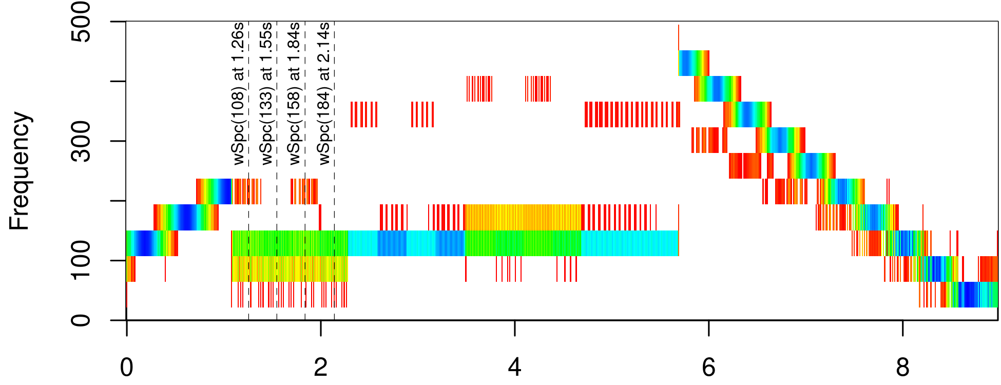
wSpec image. The unit of the x axis is seconds. The marked positions are used for the generic plot() version of tuneR in Figure 4.
Introducing rep("#DDDDDD",10) at the start of my choice of colors
turns an otherwise red background to grey. This manipulation seems to
act like noise reduction. Using only the first 67% of the rainbow
palette makes it start at red, continue with yellow, green, cyan and
end at blue. Using rainbow(200)[134:0] would reverse the palette and
begin with deep blue. Anticipating the features of
spectro() presented at the end of this section I
could also choose the spectro.colors() palette built
with the hsv() function of
grDevices. The colors are shown in the amplitude legend of
Figure 5.
In Figure 3 I marked some time spots to compare the
Wspec illustrations to the plots for the fundamental
frequencies. For comparison I picked a
boxplot() of the values used in
Figure 2. For this view I skipped the ramps. I extracted
the corresponding regions manually from the ff vector which is
developed to the time series in Section 7.4 and plotted in
Section 5. See the code below and the left
graph in Figure 4.
x <- boxplot(ts1.20[95:197],  ts1.20[198:301],
             ts1.20[302:404], ts1.20[405:490],
             main="Fundamental Freqencies\nof the Twinkle Snippet");
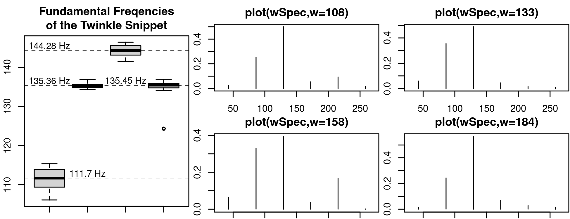
ff vector plotted in Figure 2 of Section 5. – Right: wSpec plots at the dotted time spots in Figure 3. The x axis units are Hz. These spots are correlated to the leftmost boxplot.
A specialty of R's boxplot() is its list of return values. The third line of the first list element, the x$stats matrix, contains the medians of the boxes. So I can use them for the horizontal lines, the text placement and the text itself:
abline(h=x$stats[3,],lwd=0.4,lty="dashed");
text(c(2,1,1,3),x$stats[3,],paste(round(x$stats[3,],2), "Hz"),
       a=c(0.5,-0.2),cex=0.95);
Basically the plots of my Wspec class wSpec at the chosen which'es can be invoked by the command shown in the titles of the four right graphs in Figure 4. The exact command for the first plot is
tuneR::plot(wSpec, xlim = c(30, 270), which = s[1],
            main=paste0("plot(wSpec,w=",s[1],")"));
With the distinctive features from the item list of the two Wspec
illustrations plot() and image() I think I'm ready to make my
first steps into understanding the Wspec producing
periodogram() and move to seewave's
spectro() or the much more rewarding theoretical
fields of spectral and Fourier theory. The image in Figure
5 is made without a Wspec class detour from the mono
input wnm1.20; see Section 7. It looks promising,
but the parameters and the corresponding theory are still challenging.
seewave::spectro(wnm1.20,flim=c(0,0.65));
wnm1.20 from Section 7.
Julius O. Smith [11] considers fundmental frequency
as fundamental knowledge and points to the illustrative textbook-like
entry Recognizing the Length-Wavelength Relationship at
physicsclassroom.com.22 It treats the term fundamental frequency as
the first harmonic of an instrument. So, if I aim
FF() at my wav file it selects the
fundamental frequency of the whole sound as if it was the sound of one
instrument.
Something in this class is the source for the 774 frequencies in the
resulting numerical vector of the FF() function. The
@spec list, @starts, @variance, @energy? Could be
interesting.23 I just assume that the ff vector is a number of
consecutive frequencies representing my wav snippet.
I choose another reasoning for the derivation of the vector ff. How
many samples do I need to identify the note lengths I'm looking for? I
can't find an answer to this question without the knowledge about
turning pressure values into frequency information, i.e., the mystery
of the spectral density. But I can estimate the requirements for
solving this mistery by relating the note length to the sample
rate. And then – by varying the window length – I probably can
discover some boundary values. For a \(44100\,\text{Hz}\) sampling
rate the 1024 sample window of the ff producing
periodogram() takes
In a frame of 100 BPM, i.e., 100 quarters per minute, a quarter takes \(60\,\text{s}/100=600\,\text{ms}\), a quaver \(300\,\text{ms}\), a 16th \(150\,\text{ms}\), a 32th \(75\,\text{ms}\). The window width of \(23\,\text{ms}\) is about one third of a 32th, i.e. a triplet 64th.24 The number of samples for a 32th range of \(75\,\text{ms}\) is
\begin{equation*} \frac{x}{75\,\text{ms}}=\frac{44100\,\text{samples}}{1000\,\text{ms}}; \quad \to \quad x = 3307.5\,\text{samples}. \end{equation*}
For a 16th note it would be the next integer value of 6615
samples. That fits for the Twinkle notes, the ramps would have a
coarse profile. With this estimation I could try to define a proper
overlap for 6615 samples; without leaving the pattern of the musical
beat. Anyway, the window length in the periodogram()
is restricted to \(2^{n}\) values with positive integer n exponents. The
function puts any other window size to the next \(2^{n}\) step. With
\(\log_{2}6615\approx12.7\) that would be \(2^{13}=8192\).
Armed with this information I dare to proceed using the results of FF() without knowing the internals. In the decorated twinkle case, according to str(), the result is a numerical vector of 774 elements; see Section 7.2. The values and the function name tell me that they are frequencies, but the time series information seems to be lost. Reimplementing this time information is a matter of
ts1.20 <- ts(ff, start=0, end=9, frequency=774/9);
I already used that time series for the construction of Figure 2 in Section 5 and for the boxplot in Figure 4 of Section 7.2.
In the main tuneR example the melodyplot(), the quantplot(), and a some kind of implied lilypond output are prepended by the smoother() filter. For quantplot() and lilypond there's also a quantization precursor.
For the next four subsections my mysterious notes vector of 774
elements derived with noteFromFF() from the
fundamental frequencies FF() of spectral windows
periodogram() which are calculated from the amplitude
values of my chuck recording are processed by
smoother() to snotes
The function smoother() applies moving averages – the corresponding help page talks about a “running median”. To run smoother() the user needs the additional package pastecs which, according to its help page, is aimed at “the analysis of space-time ecological series.” The borrowed function is decmedian(), “a nonlinear filtering method used to smooth, but also to segment a time series. The isolated peaks and pits are leveraged by this method.”
Reasoning about the moving average of smoother() led
me to Subsection 5.2.3 Smoothing in Section 5.2 Amplitude Envelope
of [14]'s Chapter 5 Display of the Wave. It
explains the process of a sliding window and applies it to the
concepts of moving averages, sums, and kernels mediated by the
parameters msmooth, ssmooth, and ksmooth of the
seewave function env(). The rabbit holes
I discovered in the matter of env() are
envtksmoothSo Ihave a faint idea of tuneR's smoother() function, apply it for melodyplot(), and observe its effect on the quantization methods. Perhaps I can keep in mind that seewave's env() could be a proper substitute.
snotes <- tuneR::smoother(notes);
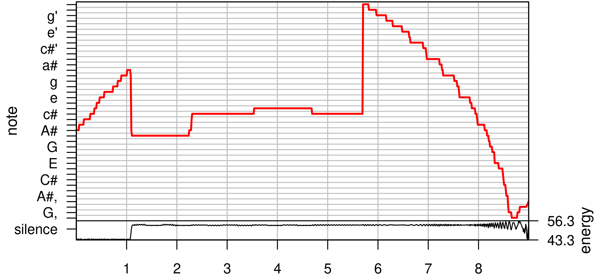
The ts class from the preceding Section 7.4 delivered the
time axis shown in Figure 2. The result in the melody
plot of Figure 6 should be pretty much the same. in
this plot the linear down slope at the end turns into a curve. That's
because of the logarithmic nature, i.e., the \(\log_{12}\) relation, of
notes and frequency. And the initial ramp doesn't have enough space on
the graph to show bending. At least I can see that the
melodyplot() is an equivalent to my self made time
series plot. The interested reader might try to substitute snotes
with notes to see some tassels.
tuneR::melodyplot(wSpec, snotes, mar=c(2,4,0,4)+0.1);
In this section is based on statements from the help page of
quantize() and quantMerge(). According to the
description both functions “apply (static) quantization of notes in
order to produce sheet music by pressing the notes into bars.” Both
read a notes vector of integers such as returned by
noteFromFF(); quantize() optionally
consumes an additional energy vector. The notes vector contains
positve and negative integer values centered about a zero note defined
by a normative frequency value called diapason.27 As
discovered in Section 3 noteFromFF()
returns an integer valued semitone difference to the diapason A3.
notes,
energy, and parts. It returns notes and energy counting
parts elements.quantMerge() responds to notes, minlength, barsize, and
bars. Its result is a data frame with the columns note,
duration, punctuation, and slur showing bars * barsize rows.
The first two lines of quantMerge() show its dependence on
quantize().
lengthunit <- bars * barsize;
notes <- quantize(notes, parts=lengthunit)$notes;
With the for-loop below I can trial and error myself through the
parts interpretation of quantize().
p <- seq(2,50,16); #p <- c(2^(2:6));
for ( i in p ) print(tuneR::quantize(snotes, wSpec@energy, parts = i));
Same experimental setup for the combination of quantMerge()'s
minlength, barsize, and bar in order to produce something useful
as input for lilypond. The definition used in
Section 7.8 is
qMnotes <- tuneR::quantMerge(notes=snotes, minlength=8, barsize=4, bar=8);
And the input for quantplot() demonstrated in
Section 7.9 is based on quantize() and uses the
energy values.
qnotes <- tuneR::quantize(snotes, wSpec@energy, parts = 64);
Table 5 shows the note values prepared by
quantMerge() and processed by a function which I borrowed from the
note-translation code28 of the function
lilyinput().
| c8 | e8 | f8 | gis8 | a,2 | cis2 | cis8 | d4. | d8 | cis4. | a'8 |
| g'8 | f'8 | e'8 | d'8 | b8 | gis8 | e8 | b,8 | e,8 | fis,,8 | gis,,8 |
After prepending and appending a half note rest r2 and adding some
slurs29 I copy & paste the result into
a lilypond template which delivers Figure 7.
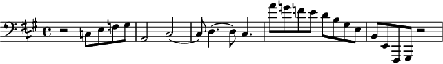
Listing1.20.ck in quaver resolution.
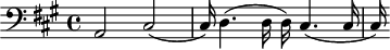
In the lilypond interpretation of the 16th resolution –
see Figure 8 – the last bass note of the melody's
accompaniment is interpreted as a half note even if it only takes 1.1
seconds; I manually split the result cis2 to cis4.(cis16
cis). Suprisingly in both the 8th and the 16th grid the second bass
note shows an abnormal length which postpones the subsequent
notes. Fortunately I can visually pre-examine the phenomenons of using
even smaller quantize() parts by the illustration
with quantplot(); see Figure 9.
The output qnotes of quantize() with 64 parts –
see Section 7.7 – is fed to
quantplot(). I present the code and the graphical
output of function without further explanation. The reader may have
collected enough inspiration to explore the 27 parameters of
quantplot() combined the parametric food of
quantize().
tuneR::quantplot(qnotes, expected=rep(c(0, -12), each=4),
                 mar=c(2,4,0,4)+0.1, bars=4)
With these tools at hand I began to translate the modules of ableton live – the live devices including instruments, audio and midi effects – into one view of sound synthesis. Another view is Peter Manning's Evolution of Sound Synthesis30. His “evolutional” sequence is, for example, wavetable synthesis → additive synthesis → frequency modulation → physical modelling → granular synthesis. And the next section of this Manning reference, 3 Resources for Software-Based Sound Synthesis, discusses plenty of tools for the tasks. The Chapter A History of Music and Programming in the chuck PhD thesis [15] offers similar insight. The thesis itself which promotes chuck as a “strongly-timed” audio programming language with a time-based concurrent programming model31 gives rise to the assumption that there's something missing in the text based sound languages nyquist and supercollider.
My experience of the terminal execution of chuck scripts
in pulse audio installations of ubuntu and
endeavoros is a hick up after about half a second of
every listing I played.32 When I record the script and play the
resulting wav file with an audio player like
vlc there's no problem. This might be an issue of my
linux configuration. Or perhaps I missed some warnings in
the compilation feedback of chuck. The chuck flag
--blocking might help but it's not available in chuck versions ≥
1.4.x. Any configuration of --bufsize didn't affect the hick up. I
didn't check --adaptive and I also didn't try to run the scripts in
audicle.
Perhaps I'd get some hints from the entry Getting an ALSA program
(ChucK) to work with Pulseaudio? and one of its references Command
line multitrack audio looper for Linux?, both at superuser.com. Or
from a 2018' phd work which expands on live coding and
classifies chuck's processing mode as a
“style of intra-process communication [which] has been adopted by many live-coding environments including chuck, impromptu and fluxus. Being both effcient and flexible, intra-process communication offers an attractive option for integrating live-coding languages with extant low-level audio-visual frameworks – opengl, stk, core-audio, quicktime, directx, alsa, jack, portaudio, and portmidi to name a few.
There is however, a serious disadvantage with the tight coupling of language with framework; the tight coupling of failure!”
— Section 3.1.2 Language and framework coupling of Extempore: The design, implementation and application of a cyber-physical programming language [12], p.47
The quote can be seen as a commercial for the extempore software, or as incentive for new ideas about live coding.
Anyway my hick up experience gives rise to the suspicion that
nyquist or supercollider are at least worth
trying. Or impromptu, fluxus,
extempore? All these software is nothing but a toolbox
for working with sound. So I might be better off to discover the
gnu linux empire which embraces the unix
philosophy of using small and highly advanced programs which are
maintainable? For example I could employ mpc, the
command-line client of the Music Player Daemon mpd for a
DJ scenario. The emacs multimedia system
emms supports it. But has emms access to the
three crossfading related flags crossfade, mixrampdb, and
mixrampdelay? What about employing SoX? Ecasound?
There are lots of programs, services, and devices which may add to an individual tool set. unix command line programs and libraries, their gui representatives, and wrappers in any coding language. Online offers and services. Looks like the users are pushed into responsibilty for their own actions. No wonder most of them decide for the proprietary thread. I voted against integrated audio software like CuBase, Magix, Rosegarden, Garageband, Muse, TuxGuitar, Frescobaldi. But I'm still interested in discovering
linux-magazine.com.That are some pieces of some big picture. But with – the recorded results of – chuck I first try the different forms of compositions from [6] and explore the live sampling expansion LiSa of chuck's sound buffer handling34 to advance my recording skills; perhaps inspiring streaming scenarios.
Even the first step can be a daunting task when I want to employ lilypond notation to drive a chuck composition. The R package tabr seems to deliver the tools for these bridges; see the initial vignette Noteworthiness: “tabr provides a music notation syntax system represented in R code and a collection of music programming functions for generating, manipulating, organizing and analyzing musical information structures in R. While other packages focus on working with acoustic data more generally, tabr provides a framework for creating and working with musical data in a common music notation format.”
And I'm also confident that my experience with notator's event handling for sequencing will be a valuable source of inspiration. Or the astonishing simplicity of notator's transform form – see Figure 10 – which is extensively discussed in the Manual [1], chapter 24, 3 Structure of the Transform Window. Looks like retro? Hmm. Guess again.

I think the very first move is employing chuck to note the events into a csv file. Or json for complex data like a glissando or a set or variables for a sound or program change. I guess both, or the good old database with normalized tables? Employing chuck should be the fastest way to a piano roll.
| I already put up an org mode file for all of tabr's elaborated vignettes. Just to understand the scope of the package. But I'm still undecided if all these tools are really helpful. For they obscure a big deal of insight if used without understanding lilypond. And lilypond in turn – for me – is a hard nut to crack either. Even if I also worked with its predecessors musictex and musixtex. So I think my entry toolset presented in this blog has still a lot to offer. |
Supplements of this blog entry: I provide the pdf here at pjs.netlify.app and a reduced version of the org source at bitbucket.org.
The online help for the installation of chuck offers
installers and source files for windows and
macos. For linux systems the help is reduced
to the statement that the library libsndfile (linked to
www.mega-nerd.com) is somehow involved and that the user should have
gcc, lex, yacc, and make; see the release page at
chuck.cs.princeton.edu. On this release page the link which says
“access all versions here” also offers a cygwin version, and the
most recent manual.
chuck-1.4.1.0 doesn't
install, chuck-1.4.0.1 works, but shows some warnings;
ubuntu itself offers the installation of version
1.2.0.8.dfsg-1.5build1, same at 2022-11-20.chuck-1.4.1.1 released in June 2022. The release page
announces that the chucK-1.4.x.x versions are part of the
NumChucKs releases of chuck which allow embedding any
number of virtual chuck machines.
| Satellite ccrma is an entire customized
version of linux that includes a number of applications
for computer music and physical computing, including
chuck. — A hint from Section
Installing on Ubuntu Linux in [6]'s Appendix A
/Installing ChucK and miniAudicle/ |
The section about the ubuntu installation in [6]'s Appendix also begins with the statement that on linux, chuck and miniaudicle are compiled from source code, but it specifies the additional programs and libraries which have to be included. The short form of the preparation is the command line expression
sudo apt-get install make gcc g++ bison flex libasound2-dev libsndfile1-dev libqt4-dev libqscintilla2-dev libpulse-dev
Another approach in ubuntu is to engage the
synaptic package manager and process each one of the
libraries and programs. They may be installed already. Check, e.g.,
which make gcc g++ at the command line of the os shell. I prefer using Sys.which() within an
r source code block to have the answer available in the
current document. I can see from the answer, that all the compilers
are installed already and accessible at 📂 /usr/bin.
Sys.which(c("make", "gcc", "g++", "bison", "flex"))
For checking the other libraries the user can chose between at least two procedures.
The first one is kind of a guess work, because the names of the
packages containing the code libraries are different in
linux flavors, like the main distributors
arch, debian, redhat, or
suse. The bash command ldconfig
configures dynamic linker run-time bindings. In linux
dynamically linked libraries are called shared objects. With the
-p flag set ldconfig prints the lists of directories and
candidate libraries stored in the current cache. In this context I
found the unix.stackexchange.com entry How Do Shared Object
Numbers Work helpful.
ldconfig -p | grep "libasound"
The second one is from askubuntu.com's entry How to find
location of installed library. The output of dpkg -L is very
long so I also piped it into grep and edited the result by
cutting some example files.
dpkg -L "libasound2-dev" | grep "libasound"
/usr/share/doc/libasound2-dev
/usr/share/doc/libasound2-dev/copyright
/usr/share/doc/libasound2-dev/examples
/usr/share/doc/libasound2-dev/examples/audio_time.c
...
...
/usr/share/doc/libasound2-dev/examples/timer.c
/usr/share/doc/libasound2-dev/examples/user-ctl-element-set.c
/usr/lib/x86_64-linux-gnu/libasound.so
/usr/share/doc/libasound2-dev/changelog.Debian.gz
As for ubuntu I can check for the installed compiler
libraries, e.g., which make gcc g++. And use the bash
command ldconfig for the run-time bindings. In arch I
add the usage of pacman -Ss for finding libasound, libsndfile,
libpulse, and qscintilla-qt4 connections; see Section Querying
Package Databases of the archwiki entry about
pacman at wiki.archlinux.org. There's probably a
similar flag or option for debian's dpkg command. One
of the pacman wrappers for arch's user
repository aur is yay. Wrappers are a subcategory of
aur helpers; “Pacman only handles updates for
pre-built packages in its repositories. aur packages are
redistributed in form of pkgbuild's and need an
aur helper to automate the rebuild process.” For my
research expanded the ldconfig-grep pipe from the
ubuntu investigation with
pacman -Ss libpulse
yay -Ss libsndfile
In 2021-09 searching for chuck on arch delivers
While the arch user repository aur provides
three packages with the gcc-libs (…) and libsndfile dependencies,
last updated at 2020-10-05: chuck-alsa, chuck-jack, and
chuck-pulse, all in version 1.4.0.1-1.
Additional aur packages for chuck are
The arch linux dependencies of the chuck installation libraries:
Mission accomplished. Now I know that I can skip qscintilla-qt4 for
my purposes.
I only use the command line invocation of audio scripts and I'm editing these scripts with emacs. For this I have to download and unpack chuck following the sequence website → Download link → source in the linux category. The download of miniAudicle is just for to check, what libraries are for the audicle and if it works. For now I'm writing documented scripts in org mode and I use the terminal or the emacs shell buffer with chuck's command line functionality. There is also a chuck shell command line interface, kind of half way to the audicle gui.
At September 2021 the arch package used 1.4.1.0 from
2021-06-25, the aur packages chuck-1.4.0.1 from
2020-04-15. Remember, at 2022-12-04 ubuntu still offers
the 1.2.0.8 version, but it takes care of the libraries. For
installation from source the tar commands below prepare for the
compilation.
tar xzf chuck-W.X.Y.Z.tgz
tar xzf miniAudicle-A.B.C.tgz
where W.X.Y.Z and A.B.C match the current version numbers. After
unpacking the user navigates to the chuck
📂 src directory of the unpacked folder system and
enters the command to start the build procedure
cd chuck-W.X.Y.Z/src
make linux-pulse
On my system make linux-alsa also works, but make linux-jack
terminates with the message
RtAudio/RtAudio.cpp:1910:10: fatal error: jack/jack.h: No such file
or directory #include <jack/jack.h> ^~~~~~~~~~~~~ compilation
terminated.  makefile:153: recipe for target 'RtAudio/RtAudio.o'
failed make: *** [RtAudio/RtAudio.o] Error 1
Perhaps a missing jack-anything-dev library; see the RtAudio header
and cpp files in RtAudio folder at chuck.cs.princeton.edu. The
make process will, again, take some time, because all of the source
code files are compiled into the single chuck program. When the
make command completes, the last step is the admin job of making the
compiled program chuck globally available.
sudo make install
I guess I could also use chuck without the sudo installer and call chuck from the
installation folder. The command chuck --version checks the availability
of chuck. I, again, process the response with
r, this time to get rid of the leading and the trailing
empty lines. Looks cumbersome, but I can control it better than the
bash source code environment in org mode. There's an R
pipe() command which probably is more convenient; it's sparsely
documented but the corresponding connections help offers a couple of
examples to learn from.
bra <- "chuck --version"; pipe <- ">";
ket <- "2>&1"; out1 <- tempfile();
rv <- system(paste(bra, pipe, out1, ket))
paste(readLines(out1)[2:5],collapse="\n")
chuck version: 1.4.0.1 (numchucks)
   linux (pulse) : 64-bit
   http://chuck.cs.princeton.edu/
   http://chuck.stanford.edu/
The org mode source code for starting a single chuck process (shred) in the emacs buffer looks like
#+header: :noeval
#+begin_src bash :exports none :results none
  chuck iCkBkEx/chapter1/Listing1.20.ck
#+end_src
I'm starting the script by disconnecting35 the :noeval header from the source code, i.e., arming
the code, and then evaluating it with C-c C-c. To stop the script I
use C-g.
| I once happended to notice a missing up-beat glissando while playing the script. But I couldn't reproduce the error on the next restart. I remember that the usage of vlc often leads to awkward behavior of the linux audio system when switching to another program. The PhD [15] only mentions internal latency problems of a sound calculation that takes longer than playing.36. |
Another mode for working with chuck code from within an org file is tangling.37 I demonstrate this feature with some short code example from the sidebox Chuck is a real programming language38 in [6]. Its realization as org mode source code block is
#+begin_src chuck :tangle ../iMuMy/Chuck/lst1p22.ck :noeval
  Impulse imp => ResonZ filt => NRev rev => dac;
  0.04 => rev.mix;
  100.0 => filt.Q => filt.gain;
  while (1) {
      Std.mtof(Math.random2(60,84)) => filt.freq;
      1.0 => imp.next;
      100::ms => now; }
#+end_src
The default way to tangle this block would be arranged with the header
argument :tangle yes. This argument in the a code block's header of
the file 📂 xx.org copies the code to
📂 xx.chuck; changing #+begin_src chuck to
#+begin_src ck leads to 📂 xx.ck; no major-mode
hacking.39 For more than one blocks in an org file with the
same target file the argument :padline controls empty line insertion
between the source blocks. Permissions for the file are set like
:tangle-mode (identity #o755). After tangling with an explicitly
given file name, like show in the code above, the script can be
processed40 with the bash command
chuck ../iMuMy/Chuck/lst1p22.ck
chuck --add
feature; I have to kill it explicitly, probably because I don't
understand the processes. And there's a lot to know, beginning with
the linux audio system and process control. As of 2018 there's a fork called chuck-mode with three elisp scripts chuck-core → chuck-console → chuck-mode at github.
The
architecture of chuck depends on kind of a client server
model. One shell provides the embracinag virtual machine which is
initialized by chuck --loop. Another shell is used for
correspondence, while the feedback is presented at the server
shell. It might be hard to provide for the corresponding control
structures in emacs. For example the function run-chuck
for starting the virtual machine is is not activated by default. The comment of the 2004 chuck-mode author: “ChucK as an internal listener does not work
well. Run it externally and control it internally.”
The audicle is designed to organize these matters. But I don't want to be gui'ded. That's why I had a hard time41 getting confidential about using the software. But I'm curious about the chuck's potential. It might be capable of concurrently controlling all kind of processes; sound design, musical composition, theatrical tonmeister processes, movie scoring, but also sonification tasks. With the control of the operating system's interfaces this can be expanded to any process control task; see the wikipedia entry about concurrency.
imho the book Programming for Musicians and Digital
Artists Creating Music with Chuck [6] offers the most
comprehensive and vivid approach for the first contact with
chuck. Unfortunately its distribution as a $30 book
doesn't meet the requirements of free software → free documentation,
unless the authors wouldn't consider their book as documentation. In
2021 the publisher offered the free chapters 0 Introduction, 3
Arrays, and 6 UGens at manning.com,42 while the program page
chuck.cs.princeton.edu links to an amazon dp
url. The examples of this book are provided in the
directory 📂 examples/book/digital-artists of the source
zip or tar 📂 chuck-1.X.Y.Z. After installation I found
it in the folder above at 📂 /usr/share/doc/chuck. It's
also mirrored at github. For free documentation the
dear reader may turn to
chuck.cs.princeton.edu, andThe other examples are planted at a structured example page. It's structure may be interpreted as a parallel view-of or approach-to chuck programming.
| [1] | C-Lab, Hamburg. Notator SL, version 3.1 edition. [ bib ] |
| [2] | Jimmie J. Cathey. Electronic Devices and Circuits. Schaum's Outline. McGraw Hill, 2011. [ bib | http ] |
| [3] | Nicolas Collins. Handmade Electronic Music: The Art of Hardware Hacking. Routledge, 2009. [ bib | http ] |
| [4] | Mitch Gallagher. Guitar Tone. Cengage Learning, 2nd edition, 2012. [ bib ] |
| [5] | Dave Hunter. Guitar Effects Pedals. Backbeat Books, 2nd edition, 2013. [ bib ] |
| [6] | Ajay Kapur, Perry Cook, Spencer Salazar, and Ge Wang. Programming for Musicians and Digital Artists. Manning Publications, 2015. [ bib ] |
| [7] | Jarmo Lähdevaara. The Science of Electric Guitars and Guitar Electronics. Books on Demand, 2012. [ bib | .html ] |
| [8] | Peter Manning. Sound synthesis using computers. In Roger T. Dean, editor, The Oxford Handbook Of Computer Music, text 4, pages 085--105. Oxford University Press, Inc., 2009. [ bib | http ] |
| [9] | Max V. Mathews, Joan E. Miller, F. R. Moore, John R. Pierce, and J. C. Risset. The Technology of Computer Music. The MIT Press, 1969. [ bib | http ] |
| [10] | Zbigniew W. Raś and Alicja A. Wieczorkowska, editors. Advances in Music Information Retrieval. Springer Berlin Heidelberg, 2010. [ bib | DOI ] |
| [11] | III. Smith, Julius O. Physical Audio Signal Processing. W3K Publishing, http://www.w3k.org/books/w3k-books, 2010. [ bib | http ] |
| [12] | Andrew Carl Sorensen. Extempore: The design, implementation and application of a cyber-physical programming language. PhD thesis, Australian National University, 2018. [ bib ] |
| [13] | S. S. Stevens, J. Volkmann, and E. B. Newman. A scale for the measurement of the psychological magnitude pitch. J Acoust Soc Am, 8:185--190, 1937. [ bib | DOI ] |
| [14] | Jérôme Sueur. Sound Analysis and Synthesis with R. Use R! Springer, 2018. [ bib | DOI | http ] |
| [15] | Ge Wang. The ChucK Audio Programming Language. PhD thesis, Princeton University, 2008. [ bib | http ] |
| [16] | E. Zwicker. Subdivision of the audible frequency range into critical bands (frequenzgruppen). J Acoust Soc Am, 33(2):248, 1961. [ bib | DOI ] |
Subsection 2.2.3 Amplitude in Section 2.2 Sound as a Mechanical Wave of [14]'s Chapter 2 What is sound?. This introduction is complemented by 18 pages of Chapter 7 Amplitude Parameterization.
Any of the emacs calculator modes
is supposed to work like invoking a calculator app from the desktop;
see the calc Manual's Section Using Calc. There's
also an org mode source code version of
calc neatly arranged with elisp – see
calc Manual's Section Calling Calc from Your Lisp
Programs – and one for org's spreadsheet feature of
tables; see org Manual's Section Formula syntax for
Calc. l s are the keys for calc-spn,
overloaded with an input integer type for midi and a
unit type in Hz or 1/s or their kilo, mega or whatever versions;
see calc Manual's Section Musical Notes. Well, some
folks might be uncomfortable with note names like Asharp_2.
His Subsection 9.4.2 Musical Scale in Section
9.4 Frequency Scales of [14]'s Chapter
Introduction to Frequency Analysis: The Fourier Transformation is
part of a two part classification in 9.4.1 Bark and Mel Scale and
9.4.2 Musical Scale. His reference for the cochlea related Bark
Scale is [16], for the psychological Mel Scale
[13]. And he points to the tuneR
function mel2hz() which works with a parameter htk
representing the Hidden Markov Model Toolkit presented at
[htk.eng.cam.ac.uk]. But these scales are more like measurement
scales.
The author calls n the rank of the note. The main
code in the function notefreq() maps the sequence
c("C", "C#", "D", "D#", "E", "F", "F#", "G", "G#", "A", "A#", "B")
or the harmonic equivalents Db, Eb, Gb, Ab, Bb to the rank
numbers 1:12 – excluding the combinations E#, Fb, B#, and
Cb. The octave index is related to pitch notation reasoning
discussed in the wikipedia entries Octave or
Scientific Pitch Notation and begins to reach into negative values
beyond C0 with \(16.35\,\text{Hz}\). It allows the user to assign a
note name to every frequency: color, γ-rays, ionization energy.
A3 is the A of the third
octave also written a'.
According to the corresponding wikipedia entry a regular staccato shortens a note by 50%. The entry quotes the music notation program Sibelius, particularly the 2008 reference manual of version 5.2.
Lilypond Learning → 1 Tutorial → 1.2 How to write input files → 1.2.1 Simple notation.
Lilypond Notation → 1 Musical notation → 1.1 Pitches → 1.1.1 Writing Piches → 1.1.1.4 Note Names in Other Languages.
ibid. → 1.1.3.1 Clef.
ibid. → 1.1.3.2 Key Signatures.
ibid. → 1.2 Rhythms → 1.2.3 Displaying Rhythms → 1.2.3.2 Metronome Marks.
ibid. → 1.5 Simultaneous notes → 1.5.2 Multiple Voices → 1.5.2.6 Writing Music in Parallel. The the trigger symbol for this parallel notation is the vertical line.
At
lilypond's github repository in the
📂 lilypond/elisp/ folder or mjago's
emacs repo in the 📂 lilypond/
folder.
Lilypond Notation → 4 Spacing Issues → 4.3. Breaks → 4.3.2 Page Breaking → 4.3.2.5 One-line Page Breaking.
ibid. → 3 General input and output → 3.2 Titles and headers → 3.2.2 Custom titles, headers, and footers → 3.2.2.2 Custom layout for titles and 3.2.2.3 Custom layout for headers and footers.
In later versions the lilypond part of this section will be supplemented significantly by the exploration of the R package tabr.
In Subsubection 13.1.2.2 tuneR Solutions, Subsection 13.1.2 Fundamental Frequency, Section 13.1 Frequency Tracking, of [14]'s Chapter 13 Frequency and Energy Tracking.
The author calls FF() a
wrapper of FFpure() and links it to the short-time discrete Fourier
transform (stdft) matrix. “A good way to understand how
stdft works is to use the interactive function
dynspec(). The function computes a
stdft and displays the successive
dfts. […] The stdft is by essence a
collection of successive frequency spectra that are grouped into a
single matrix which dimensions are determined by the length N of the
sound and the time index m that corresponds to the size of the
sliding window”; see the Subsection 11.1.1 Principle of Section
11.1 Short-time Fourier Transformation in
[14]'s Chapter 11 Spectrographic
Visualization. dynspec() is a seewave
function which requires rpanel.
The package
offered a very detailed vignette about Acoustic Analysis, removed
at 2022-12-10 from the cran repository due to updated
package size restrictions. The reader might be lucky to still find
it as a snapshot at mran.microsoft.com.
See Default Channel
Ordering in the Multiple channel audio data and WAVE files entry at
learn.microsoft.com for a working link, accessed 2023-01-28.
Subsection Recognizing the
Length-Wavelength Relationship → Section Fundamental Frequency and
Harmonics → Lesson 4 Resonance and Standing Waves in Physics
Tutorial's Chapter Sound Waves and Music at
physicsclassroom.com.
Apart from being confronted with psd and
dft realms (see below) a possible entry into the rabbit
hole is Section 11.4 Functions of the Package tuneR in
[14]'s Chapter 11 Spectrographic
Visualization, p. 321f: “The most important slot is the slot @spec
which contains the successive power spectrum densities
(psd's) organized in a list. […] To get a display of
the spectrogram, we need to extract the slot @spec, to convert it
into a matrix, to scale the data in \([0,1]\), to convert the data in
dB, and to use the function 2D-plot function
image() to plot the transpose of the
matrix. Labeling the axes is a bit tricky, in particular for the time
axis.” There's another entry at Subsection 10.1.1 Functions of the
Package tuneR in 10.1 Frequency Spectrum of
[14]'s Chapter 10 Frequency, Quefrency, and
Phase in Practice, p.248f: “The function
periodogram() of tuneR, which is based on
spec.pgram() from the R core package
stats, computes the power spectral density (PSD) which
is the square of the frequency spectrum of the discrete Fourier
transform dft. The frequency spectrum is scaled by the
sum of the dft values returning therefore a probability
mass function.”
The question is what would be a serious resolution? That depends. For the continuous up and down ramps it might have to be as small as possible, and for the quaver notes a 16th resolution might suffice. But looking at the procedural data of an up or down ramp we only need the start and end note, the ramping time, and perhaps a ramping profile. The profile would describe the pattern to get from start to end; linearly, sinusodially increasing, whatever. The glissando notation includes this freedom of interpretation.
The main example of tuneR uses
smoother()'ed snotes for the
quantize() input. But as far as I've seen the usage
of notes yields the same result.
The timer() function is central to the 13-page section 8.3 Automatic Measurements in [14]'s Chapter 8 Time-Amplitude Parametrisation. This is 13 pages about looking for relevant signals in a sea of noise or silence just by applying a threshold. the whole 30-page-chapter Comparison and Automatic Detection of the same book treats pattern matching.
Diapason is short for diapason normal correlated to the concert pitch.
Because of its length the code is not shown,
but it's part of this blog's org file. The dear reader
may also look up the part in the lilyinput()
function. Its the part from the assignment of clef to the return
value statement toene. I consider this note decoder as the central
part of this lilyinput() function.
Some notes are split automatically in order to comply to the musical beat structure. These breaks are then rebound with a slur. This slur provision is already announced for the lilyinput() function.
I also checked this behavior in a real terminal of an ubuntu system, i.e., the terminal which is usually available via C-M-F1 to C-M-F?, not the terminal emulations of the graphical desktop.
Direct Link chosen from an
overview of Sound Examples in one of his online publications
Physical Audio Signal Processing at www.dsprelated.com or at
ccrma.stanford.edu. Both example sections are pointing to
wav and mp3 files at
ccrma.stanford.edu.
Connecting the
#+header: after playing is a good habit for avoiding the org-lint
message “orphaned header argument,” but I didn't hear the code
executed at any export without the :noeval header. Well, :exports
and :results are both set to none; see the org
Manual's Section Evaluating Code Blocks for their effect on
evaluation.
See the “two points should be noted” in Subsection 3.4.3 ChucK Virtual Machine + Shreduler, Section 3.4 System Design and Implementation of [15]'s ChucK Chapter, p.78.
See Section Extracting Source
Code of the org Manual or the docstring of
org-babel-tangle, shortcut C-c C-v t.
The sidebox is part of Section 1.2.3 Now
let’s make music, Section 1.2 Your first ChucK programs of
[6]'s first Chapter Basics: sound, waves, and ChucK
programming, p.22. The purpose of the sidebox is the demonstration of
a short loop to create an infinite number of sounds in contrast to the
tedious task of explicitly creating four Twinkle notes in
📂 Listing1.2.ck.
Usage of :comments will involve more configurational
effort, because the default comment markup probably won't fit for
chuck code. The argument :comments org transfers parts
of the org document to the code file, while :comments
link inserts backlinks in the code file to the org
file.
In chuck parleur: the shred can be sporked to the vm.
Took me some time to see the SndBuf's dependence on
linux's \(48\,\text{kHz}\) default. For access to
external wav files I have to reduce the sampling rate
with chuck --srate44100, not --srate:44100 or --srate(44100) in
commands of the client terminal. I noticed that while referring to
wav snippets located by audacity. With the
linux default chuck couldn't find these
pieces using \(44.1\,\text{kHz}\) audacity's sample
locators.
In 2023-02 the visitor gets a time window for providing an email address.